3  Methods

This section describes how we construct a model of access to grocery stores in communities in Utah. We first describe the theoretical model, and then describe data collection efforts to estimate this model and apply it.

3.1 Model

A typical model of destination choice (Recker & Kostyniuk, 1978) can be described as a random utility maximization model where the utility of an individual i choosing a particular destination j is U_{ij} = \beta_{s}f(k_{ij}) + \beta_{x}(X_j) \tag{3.1} where f(k_{ij}) is a function of the travel impedance or costs from i to j and X_{j} represents the location attributes of j. The coefficients \beta can be estimated given sufficient data revealing the choices of individuals. The probability that individual at location i will choose alternative j from a choice set J can be estimated with a multinomial logit model (MNL) (McFadden, 1974), P_i(j) = \frac{\exp(U_{ij})}{\sum_{j' \in J}{\exp(U_{ij'})}} \tag{3.2} The overall fit of the model can be described with the Akaike Information Criterion (AIC) — which should be minimized — or by the McFadden likelihood ratio \rho^2_0 = 1 - \ln\mathcal{L} / \ln\mathcal{L}_0. In this ratio \ln{\mathcal{L}} is the model log-likelihood and \ln{\mathcal{L}_0} the log-likelihood of an alternative model where all destinations are equally likely; a higher \rho^2_0 value indicates more explanatory power relative to this null, random chance only model.

The idea of using destination choice logsums as accessibility terms is not new, and the theory for doing so is described in Ben-Akiva & Lerman (1985, p. 301). Effectively, the natural logarithm of the denominator in Equation 3.2 represents the consumer surplus — or total benefit — available to person i:

CS_i = \ln\left(\sum_{j \in J} \exp(U_{ij})\right) \tag{3.3}

A difference in logsum measures may exist for a number of reasons that affect the utility functions described in Equation 3.1. For example, individuals at different locations or with different mobility will see different impedance values k_{ij} and therefore affected utility. Changes to the attributes of the destinations X_j will likewise affect the utility.

Despite the relative maturity of this theory, applications of utility-based access in the literature are still rare, outside of public transport forecasting analyses (Geurs et al., 2010). The rarity is likely explained by an unfamiliarity with destination choice models and the ready availability of simpler methods on one hand (Logan et al., 2019), and the difficulty in obtaining a suitable estimation dataset for particular land uses on the other (Kaczynski et al., 2016). This second limitation has been somewhat improved by a new methodology developed by Macfarlane et al. (2022) , relying on commercial location-based services data to estimate the affinity for simulated agents to visit destinations of varying attributes and distances.

3.2 Data

In this research, we develop a unique dataset to estimate the destination choice utility coefficients for grocery store choice in three different communities in Utah. The three communities were selected to maximize potential observed differences in utility between community residents. The three communities are Utah County, West Salt Lake Valley, and San Juan County. Note that in this document we refer to the second community as “Salt Lake” even though this does not refer to the entire Salt Lake County nor to Salt Lake City, rather, we focus on communities in the western part of the valley, such as Magna, Kearns, and West Valley City.

Table 3.1 shows several key population statistics based on 2021 American Community Survey data for block groups in the three communities of interest. Utah County is a largely suburban county with high incomes and a low percentage of minority individuals. The Salt Lake region is more dense with somewhat lower incomes and household sizes but a high share of minority individuals. San Juan County is primarily rural, with a few small communities and a large reservation for the Navajo Tribe.

tar_load(neighbor_acs) 
df <- neighbor_acs |> 
  mutate(county = relevel(factor(county), ref = "Utah")) |> 
  group_by(county) |> 
  summarise(
    `Total population` = sum(population),
    `Total households` = sum(households),
    `Housing units per sq. km` = weighted.mean(density, housing_units),
    `Median income` = Hmisc::wtd.quantile(income, weights = households, probs = .5),
    `Percent minority individuals` = weighted.mean(100 - white, population)
  ) |> 
  data.table::transpose(make.names = 'county', keep.names = 'measure')

if(!knitr::pandoc_to("docx")){
  kbl(df, col.names = c("", "Utah", "Salt Lake", "San Juan"), digits = 0, 
      format.args = list(big.mark = ','), booktabs = TRUE) |> 
  kable_styling()
}
Table 3.1: Demographic Statistics of Study Region
Utah Salt Lake San Juan
Total population 627,098 655,830 7,091
Total households 171,538 216,731 2,090
Housing units per sq. km 599 831 103
Median income 79,453 64,868 58,586
Percent minority individuals 18 36 26

Estimating the utility model described in Equation 3.2 for grocery stores requires three interrelated data elements:

  1. an inventory of grocery store attributes X_j,
  2. a representative travel impedance matrix K composed of all combinations of origin i and destination j.
  3. a database of observed person flows between i and j by which to estimate the \beta coefficients.

We describe each of these elements in turn in the following sections.

3.2.1 Store Attributes

tar_load(nems_groceries)

The store attributes were collected using the Nutritional Environment Measures Survey — Stores (NEMS-S) tool (Glanz et al., 2007). This tool was developed to reveal significant differences in the availability and cost of healthy foods in an environment, and has been validated for this purpose. Beyond superficial attributes such as the store category (dollar store, convenience store, ethnic market, etc.) and the number of registers, the NEMS-S collects detailed information about numerous store offerings such as the availability of produce, dairy products, lean meats, juices, and canned and dry goods of various specific types. Of particular interest to the survey are availability and price differentials of lower-fat alternatives: for example, the survey instrument requests the shelf space allocated to milk products of various fat levels and the price of each product.

Student research assistants collected the store attributes by visiting grocery stores, dollar stores, ethnic markets, and other food markets in the three communities of interest described above. Stores were identified using internet-based maps combined with in-person validation and observation. The student researchers completed the NEMS-S instrument with the aid of a digital survey and a tablet computer. Each researcher who collected data was trained to use the survey at a control store in Provo, and the training data helped to eliminate the risk of surveyor bias. The store attributes were collected in the spring of 2021 for Utah County and spring of 2022 for Salt Lake and San Juan Counties. In Utah and Salt Lake Counties, we included dollar stores and grocery stores but did not include convenience stores. Given the rural nature of San Juan County, we made two adjustments to capture the entirety of the nutrition environment. First, we included convenience stores and trading posts if they were the only food market in a community. We also included full-service grocery stores in Cortez, Colorado, and Farmington, New Mexico in the San Juan data collection, as community conversations made it clear that many residents will drive these long distances for periodic shopping with greater availability and lower prices.

Using the information in the NEMS-S survey, two measures of a store can be calculated: an availability score based on whether stores stock particular items as well as lower-calorie options; and a cost score describing the spread between prices of these options. These score values are described in Lunsford et al. (2021), and we developed an R package to compute the scores; this package is available at https://github.com/byu-transpolab/nemsr. In the availability score each store is given a value for whether or not there are more healthful options available in the store, such as low-calorie chips, or low-fat milk. If the store does not have a more healthful option in a category it receives a lower score, so stores with more availability of healthful food options will receive a higher availability score. For the cost score, the measure is the price spread between healthful and less healful options: if the price of whole wheat bread is cheaper than white bread, the store receives positive points for the cost option, if the price is the same then zero points are awarded, and if the wheat bread is more expensive then the store receives negative points. Thus a store with a higher availability and cost score will have both more healthful options, and a more advantageous pricing scheme towards those options.

One important store attribute that the NEMS-S instrument does not collect or compute directly is a measure of the cost of common goods that can be compared across stores. We therefore used the data collected from the NEMS-S instrument to construct a market basket-based affordability measure that could be compared across stores, following the approach of Hedrick et al. (2022). This market basket score is based on the US Department of Agriculture (USDA) 2021 Thrifty Food Plan (FNS, 2021), which calculates a reference market basket for a family of four. Because this market basket contains more (and sometimes different) items than what the NEMS-S instrument requests, we chose relevant items from our NEMS-S data as replacements. For example, the USDA market basket contains a certain amount of poultry, but the NEMS-S score collects the per-pound cost of ground beef at various fat contents. For any stores that were missing any of the elements in the market basket, we first substituted with another ingredient that would fit the nutritional requirements. If no substitute was available, we included the average price of the missing good at other stores in that community multiplied by 1.5 as a penalty for not containing the product. The final market basket score is the total cost of all foods in the market basket. These costs can then be compared from store to store to understand general affordability comparisons between stores.

tar_load(nems_groceries)

balnems <- nems_groceries |> 
  ungroup() |> 
  transmute(Type = ifelse(type == "Trading Post", "Other", type),
            Pharmacy = pharmacy, 
            `Ethnic market` = ethnic,
            `Other merchandise sold` = merch, 
            `Registers (incl. self checkout)` = total_registers,  
            `NEMS-S availability score` = availability, 
            `NEMS-S cost score` = cost, 
            `Market basket cost` = market, 
            County = factor(county, levels = c("Utah", "Salt Lake", "San Juan")))

if(!knitr::pandoc_to("docx")){
  datasummary_balance(~County, data = balnems) |> 
    kable_styling(latex_options = "scale_down")
}
Warning: Please install the `estimatr` package or set `dinm=FALSE` to suppress
this warning.
Table 3.2: Grocery Store Attributes
Utah (N=63)
Salt Lake (N=39)
San Juan (N=50)
Mean Std. Dev. Mean Std. Dev. Mean Std. Dev.
Registers (incl. self checkout) 12.5 11.7 9.9 8.9 6.1 8.8
NEMS-S availability score 18.7 8.4 16.2 8.1 13.2 7.6
NEMS-S cost score 1.9 2.3 2.3 2.2 1.9 1.9
Market basket cost 126.1 21.5 141.6 19.2 157.6 16.8
N Pct. N Pct. N Pct.
Type Convenience Store 2 3.2 0 0.0 10 20.0
Dollar Store 5 7.9 11 28.2 15 30.0
Grocery Store 50 79.4 27 69.2 19 38.0
Other 6 9.5 1 2.6 6 12.0
Pharmacy FALSE 42 66.7 32 82.1 43 86.0
TRUE 21 33.3 7 17.9 7 14.0
Ethnic market FALSE 55 87.3 30 76.9 47 94.0
TRUE 8 12.7 9 23.1 3 6.0
Other merchandise sold FALSE 52 82.5 35 89.7 47 94.0
TRUE 11 17.5 4 10.3 3 6.0

Table 3.2 presents the store attribute data collected for each community. Utah County generally has the largest average store size (as measured by the number of checkout registers) while having the lowest market basket cost, the highest availability of health food (the NEMS-S availability score) and the lowest difference between healthy and unhealthy food (the NEMS-S cost score). San Juan County has the smallest average stores, highest costs and the lowest availability of healthy options, and Salt Lake falls in between.

3.2.2 Imputation of Missing Store Data

We collected detailed store attributes for stores in Utah County, San Juan County, and a portion of Salt Lake County using the NEMS-S survey instrument. These attributes form the basis of the choice models used to determine access, but understanding access in other parts of Salt Lake City or the state of Utah requires us to impute the attributes onto the stores that we did not collect.

To do this, we used web-based mapping databases (including OpenStreetMap and Google Maps) to obtain a list of grocery stores, dollar stores, and appropriate convenience stores throughout the state. From this search, we were able to determine each store’s location, brand name, and store type, which we also collected in the manual data assembly efforts. Using this information, we built a multiple imputation model using the mice package for R (van Buuren & Groothuis-Oudshoorn, 2011). The predictor variables in the imputation included the store brand and type, as well as the average income and housing density in the nine closest block groups to the store location (based on population-weighted centroids).

tar_load(imputed_groceries)
combined <- lapply(seq_along(imputed_groceries), 
                   function(i) mice::complete(imputed_groceries, i)) |> 
  bind_rows(.id = "imputation") |> 
  filter(type == "Grocery Store") |> 
  as_tibble()

sampled_store_ids <- sample(combined$id, 15)
set.seed(42)
combined |> 
  filter(id %in% sampled_store_ids) |> 
  filter(!grepl("SL|UT|SJ", id)) |> 
  arrange(id) |> 
ggplot(aes(x = market)) +
  geom_density() + facet_wrap(~id) + theme_bw() +
  xlab("Imputed Market Basket Price [$]") + 
  ylab("Density")

Figure 3.1: Imputed market price values for 15 random grocery stores.

Thirty iterations of the multiple imputation algorithm were run for each of ten independent imputations. Figure 3.1 shows the density of the ten imputed market basket prices for a randomly selected set of 15 stores. As the figure reveals, there is some general peaking in the predicted market price for most stores, but the imputation model still predicts a wide range of possible prices for most stores. When using the imputed data for analysis, we take the mean of the ten predictions for continuous values, and the mode for discrete values.

3.2.3 Travel Impedances

The second element of the utility equation in Equation 3.1 is the travel impedance between i and j. Many possibilities for representing this impedance exist, from basic euclidean distance to complex network paths. A primary purpose of the model we are developing in this research is to study comparative tradeoffs between infrastructure-focused and environment-focused improvements to the nutrition access of households. It is therefore essential that we use a travel impedance measure that can combine and compare the cost of traveling by multiple modes so that highway improvements and transit / active transport improvements can be compared in the same basic model.

tar_load(utilities)

Just as the log-sum of a destination choice model is a measure that sums the utility of multiple destination attributes and costs in a rigorous manner, the log-sum of a mode choice model combines the utilities of all available travel modes. In this study we assert the following mode choice utility equations: \begin{align*} V_{\mathrm{auto}, ij} &= -0.028(t_{\mathrm{auto}, ij})\\ V_{\mathrm{bus}, ij} &= -4 -0.028(t_{\mathrm{bus}, ij}) -0.056(t_{\mathrm{wait}, ij}) -0.056(t_{\mathrm{access}, ij})\\ V_{\mathrm{walk, ij}} &= -5 -0.028(t_{\mathrm{walk}, ij}) -1.116(d_{ij<1.5}) -5.58(d_{ij>1.5})\\ \end{align*} where t is the in-vehicle travel time in minutes for each mode between i and j. The transit utility function additionally includes the wait time for transit as well as the time necessary to access the transit mode on both ends by walking. The walk utility includes a per-mile distance disutility that increases for distances greater than 1.5 miles. These equations and coefficients are adapted from a statewide mode choice model developed for UDOT research (Barnes, 2021).

The log-sum, or total weighted impedance by all modes is therefore k_{ij} = \ln(e^{V_{\mathrm{auto}, ij}} + e^{V_{\mathrm{bus}, ij}} + e^{V_{\mathrm{walk},ij}}) \tag{3.4}

In this implementation, i is the population-weighted centroid of a 2020 Census block group, and j is an individual grocery store. We measure the travel times from each i to each j using the r5r implementation of the R5 routing engine (Conway et al., 2017, 2018; Conway & Stewart, 2019; Pereira et al., 2021). This algorithm uses common data elements — OpenStreetMap roadway and active transport networks alongside General Transit Feed Specification (GTFS) transit service files — to simulate multiple realistic route options by all requested modes. We obtained OpenStreetMap networks and the Utah Transit Authority GTFS file valid for May 2023 and requested the minimum total travel time by each mode of auto, transit, and walking for a departure between 8 AM and 9 AM on May 10, 2023. The total allowable trip time by any mode was set to 120 minutes, and the walk distance was capped at 10 kilometers; if a particular i,j pair exceeded these parameters then the mode was presumed to not be available and contributes no utility to the log-sum.

3.2.4 Mobile Device Data

The final element of destination utility presented in Equation 3.1 are the coefficients, which are often estimated from household travel surveys in a travel demand context. It is unlikely, however, that typical household diaries would include enough trips to grocery stores and similar destinations to create a representative sample.

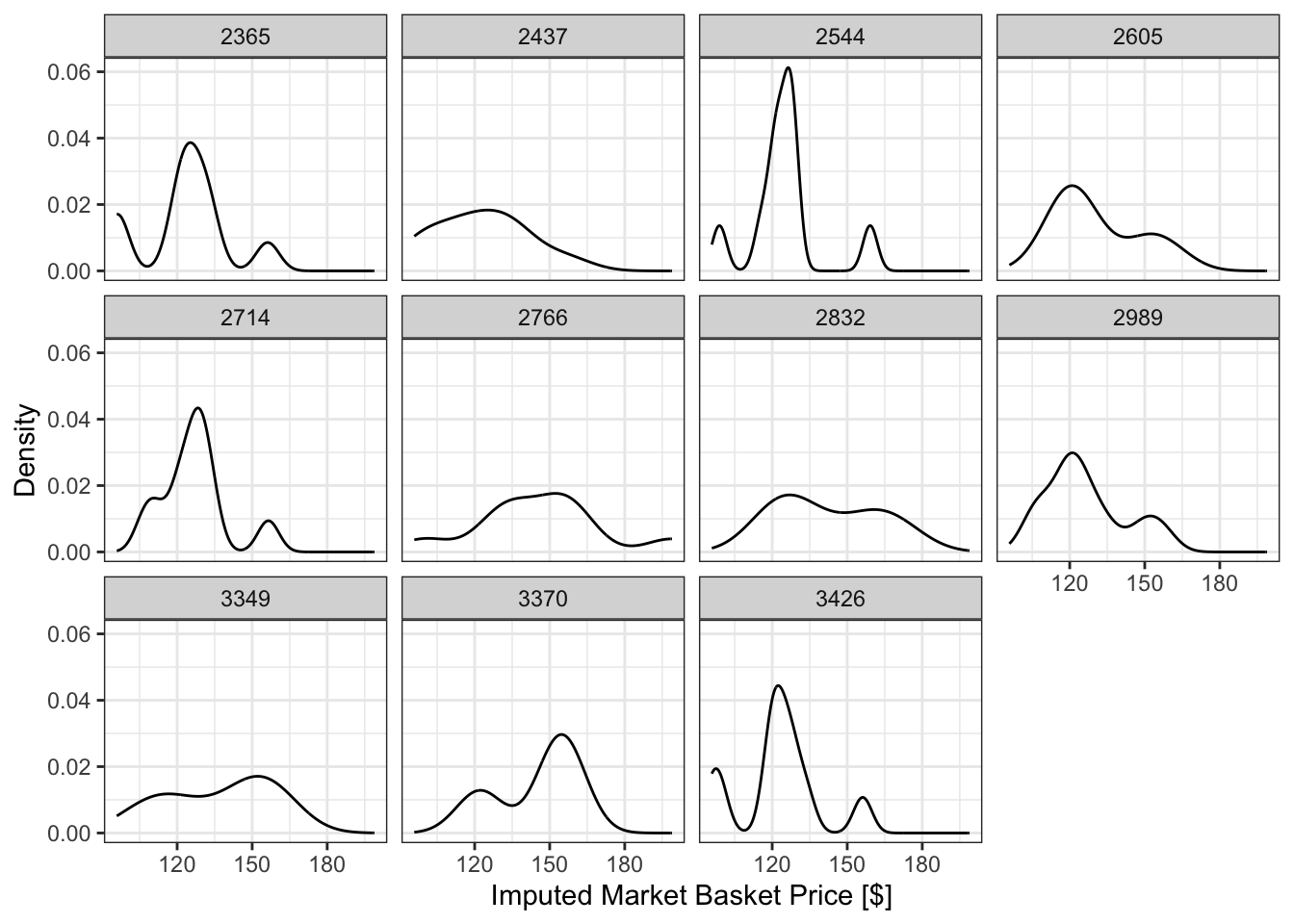
Emerging mobile device data, however, could reveal the typical home locations for people who are observed in the space of a particular store. Macfarlane et al. (2022) present a method for estimating destination choice models from such data, which we repeat in this study. We provided a set of geometric polygons for the grocery stores of interest to StreetLight Data, Inc., a commercial location-based services aggregator and reseller. StreetLight Data in turn provided data on the number of mobile devices observed in each polygon grouped by the inferred residence block group of those devices during summer 2022. We then created a simulated destination choice estimation dataset for each community resource by sampling 10,000 block group - grocery store “trips” from the StreetLight dataset. This created a “chosen” alternative; we then sampled ten additional stores from the same community at random (each simulated trip was paired with a different sampled store) to serve as the non-chosen alternatives. Random sampling of alternatives is a common practice that results in unbiased estimates, though the standard errors of the estimates might be larger than could be obtained through a more carefully designed sampling scheme (Train, 2009).