A Demonstration Model
In this class we will use the model for the Roanoke Valley Transportation Planning Organization (RVTPO), the MPO responsible for transportation planning in Roanoke, Virginia. The model is written for the CUBE travel modeling software package, the same software used by the Wasatch Front Regional Council model. The model code and files are available on Box.
A few key parameters files have been reset to default values, rather than the calibrated values used in the actual model. The homework assignments and lab activities in this course will walk you through re-calibrating the model to use in your term assignments.
A.1 Running the Model
The model files are available f rom Box
as a compressed file called rvtpo_bare.zip. Extract this file to a folder on
your local computer. I prefer to keep my models in a
folder on the C:\ drive called C:\projects. It may be that the C drive is
not available to you, but you should place the model at a path that makes sense
and that will not change from session to session. It is possible that the J:
drive will not have enough space for multiple runs of the model.
The path that you choose must have no spaces, from the drive letter to the final folder, i.e.,
C:\folder\folder\rvtpo_bare. If there are any spaces your model will crash.

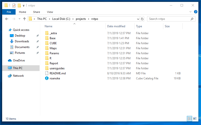
Figure A.1: RVTPO model home folder
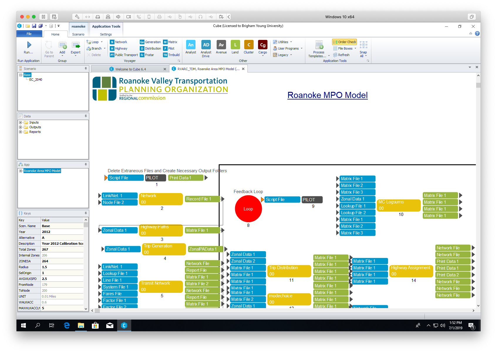
Double-click on the roanoke.cat Cube catalog file. This will open
the model application interface in Cube. On this interface you can see the steps
the model will execute, as well as access the input / output files for each
step. Some steps actually contain several sub-steps, and double-clicking the
yellow step box will expand that application.

Figure A.2: RVTPO model application interface
Run the base scenario of the model by pushing the large blue “Run”
button in the upper left-hand corner of the Cube application. A window
will appear first asking you to confirm which scenario you are running, and then
showing you the progress. This model takes approximately 15 minutes to run on my
laptop.9 Complete instructions are included in the model user’s guide (in the
usersguide/ folder).
I have also made a YouTube video showing these steps. Note that the video shows you getting the model from Canvas; get it from Box.
A.2 Files and Reports
You can access files in the model in multiple ways:
- Through the application manager in Cube (input / output boxes)
- In the catalog windows on the side
- Directly in the File Explorer
The model has a few prepared reports that you can run at any time. These are found in the “Reports” drop-down in the catalog along the left-hand side of the Cube window. These reports include:
- Highway vehicle miles traveled and vehicle hours traveled by facility type
- Mode choice by purpose
- Transit route-level boardings in Peak and Off-peak periods
You can also make tabulations of any report. The video below has an example.
A.3 Writing Custom Scripts
Sometimes what you would like to look at is not calculated directly from the model, but you can write scripts that will compute what you need. Two common script types are for matrix manipulation and for network manipulation.
A.3.1 Network Bandwidth
The script below will compute the difference between 2040 and 2012 highway volumes. The script can be adapted for similar applications. The video shows how to use this script and calculate what you need to.
RUN PGM=NETWORK
NETI[1] = "C:\projects\rvtpo-master\Base\Output\LOADED_2012A.net"
NETI[2] = "C:\projects\rvtpo-master\Base\EC_2040\Output\LOADED_2040A.net"
NETO = "C:\projects\rvtpo-master\Base\Output\Growth.net" INCLUDE = base_vol, ec2040_vol, diff

PROCESS  PHASE=INPUT
;Use this phase to modify data as it is read, such as recoding node numbers.
ENDPROCESS

PROCESS  PHASE=NODEMERGE
; Use this phase to make computations and selections of any data on the NODEI files.
ENDPROCESS


PROCESS  PHASE=LINKMERGE
  ; Use this phase to make computations and selections of any data on the LINKI files.
  base_vol = li.1.TOTAL_VOL
  ec2040_vol = li.2.TOTAL_VOL
  diff = ec2040_vol - base_vol
ENDPROCESS

PROCESS  PHASE=SUMMARY
; Use this phase for combining and reporting of working variables.
ENDPROCESS

ENDRUN
A.4 Network and Zone Maps
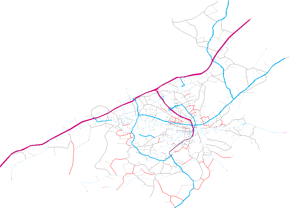
You can use Cube to create maps of network and zone data that you can use for debugging and analysis. You can also include these graphics in reports and presentations. For example, Figure A.3 shows the network links by facility type. The video below shows how to do this.

Figure A.3: Facility types in the Roanoke region.
A.4.1 Shortest Paths
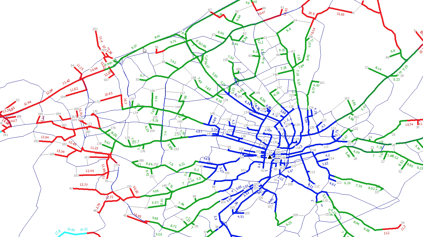
You can use Cube to measure the shortest path between two points in your model network. You can also make isochrone maps of the travel time to various destinations from a specific origin point, like the map shown in Figure A.4. The video below shows how to do this.

Figure A.4: Isochrone map using network speed information.
A.4.2 Mode Choice Logsum Maps
The mode choice model logsums are an important accessibility component in the model that you may want to visualize. This video shows how to create these datasets and visualize them.
The script is here:
/*
  Average logsum calculator

  This script reads in a matrix (ideally a logsum) matrix and writes out the row averages.
*/
RUN PGM=MATRIX

  ; Input matrix 1
  FILEI MATI[1] = "C:\projects\rvtpo-master\Base\Output\HBW_MCLS.MAT"
  ; Can add additional input matrices
  FILEI MATI[2] = "C:\projects\rvtpo-master\Base\Output\HBO_MCLS.MAT"

  ; Output DBF
  FILEO RECO[1] = "C:\projects\rvtpo-master\Base\Output\average_mcls.dbf",
        FIELDS= Z HBW HBO ; can add additional fields

  ; specify which working matrices are which purpose
  ; MW[n] = MI.[which mati].[which table]
  FILLMW MW[1] = MI.1.1 ; HBW
  FILLMW MW[2] = MI.2.1 ; HBO
  ; can add additional fields


  ; The MATRIX program has an implicit row loop. So for each row, we restart the N and sum calculations
  n = 0
  hbw = 0
  hbo = 0

  ; loop through destinations
  LOOP JJ=1, ZONES
    hbw = hbw + MW[1][JJ]
    hbo = hbo + MW[2][JJ]
    ; add other fields
    n = n + 1 ; increment number of zones
  ENDLOOP

  ; write output record
  RO.Z = I
  RO.HBW = hbw / n
  RO.HBO = hbo / n
  ; other fields

  WRITE RECO = 1


ENDRUNIt’s a small model with only about 250 zones; a larger model like WFRC will take many hours. Generally model run time increases with the square of the zones.↩︎