3 Results
The surveyors conducted 55 interviews in the first tranche and 75 in the second tranche; the second tranche consisted of 58 interviews on rail transit platforms and 17 interviews on the mictrotransit vehicles or at the microtransit pick-up point adjacent to the rail stations. A summary of the survey respondents in each tranche is given in Table 3.1; as outlined in the Methodology section, the decision to include income level in the survey was made between the tranches and therefore the “Before” tranche contains no income information. The number of respondents who declined to answer the other demographic questions is also high.
datasummary_balance(
    ~ tranche,
    survey_data %>%
        transmute(
            tranche,
            Smartphone = fct_explicit_na(phone),
            `Household size` = fct_explicit_na(size_cat),
            Age = fct_explicit_na(age),
            `Auto availability` = fct_explicit_na(autos),
            Income = fct_explicit_na(income),
            `Weekly transit use` = fct_explicit_na(frequency_cat)
        ),
    title = "Demographic Characteristics of Survey Respondents"
)| N | % | N | % | ||
|---|---|---|---|---|---|
| Smartphone | No | 3 | 2.3 | 2 | 1.5 |
| Yes | 42 | 32.3 | 48 | 36.9 | |
| (Missing) | 10 | 7.7 | 25 | 19.2 | |
| Household size | 1 | 0 | 0.0 | 4 | 3.1 |
| 2 | 0 | 0.0 | 10 | 7.7 | |
| 3 | 0 | 0.0 | 7 | 5.4 | |
| 4+ | 0 | 0.0 | 29 | 22.3 | |
| (Missing) | 55 | 42.3 | 25 | 19.2 | |
| Age | Under 18 | 0 | 0.0 | 3 | 2.3 |
| 18-24 | 12 | 9.2 | 8 | 6.2 | |
| 25-44 | 24 | 18.5 | 28 | 21.5 | |
| 45-64 | 9 | 6.9 | 10 | 7.7 | |
| Over 65 | 0 | 0.0 | 1 | 0.8 | |
| (Missing) | 10 | 7.7 | 25 | 19.2 | |
| Auto availability | 0 | 0 | 0.0 | 4 | 3.1 |
| 1 | 18 | 13.8 | 19 | 14.6 | |
| 2 | 13 | 10.0 | 18 | 13.8 | |
| 3 | 8 | 6.2 | 8 | 6.2 | |
| 4+ | 3 | 2.3 | 5 | 3.8 | |
| (Missing) | 13 | 10.0 | 21 | 16.2 | |
| Income | Less than $44,999 | 0 | 0.0 | 8 | 6.2 |
| $45,000 to $100,000 | 0 | 0.0 | 17 | 13.1 | |
| Over $100,000 | 0 | 0.0 | 17 | 13.1 | |
| (Missing) | 55 | 42.3 | 33 | 25.4 | |
| Weekly transit use | One day or less frequently | 8 | 6.2 | 13 | 10.0 |
| Two to four days | 22 | 16.9 | 37 | 28.5 | |
| Five days or more | 25 | 19.2 | 25 | 19.2 |
A primary motivation for the survey was to understand awareness of the microtransit service among UTA transit riders. In the “Before” tranche, only 6 of the 55 respondents (11%) stated they had previously heard of the system. Of the 58 interviews in the “After” tranche not conducted on the microtransit service, 34 (59%) had previously heard of the service. This increase in general awareness of the system indicates both that the UTA marketing efforts were effective, and also that the responses to the subsequent question of likeliness to use the service are based in some level of understanding.
Figure 3.1 shows the reported likelihood of survey respondents to download the necessary application and use the microtransit service, separated by access mode. Respondents who were already using the service selected “5: Extremely Likely.” The first result of this analysis is that there appears to be a polarization in opinions after the service commenced operations. Although there are some strong feelings against and for the service in the “Before” tranche, the neutral opinions have comparatively disappeared in the “After” tranche. This likely reflects the increasing awareness of the service discussed above and a hardening of ingrained or newly learned habits. It is important also to stress that the question will not necessarily elicit an opinion as to whether the service should exist, merely whether the particular respondent is willing to use it.
The sample is too small to conduct meaningful statistical inference on the role that access mode plays in these opinions, but some discussion of these observations is still worthwhile. The apparent reluctance of bicyclists to use the service is likely statistical noise, though it should also be noted that the “After” tranche was collected in January and February, when Utah is typically cold with snow on the ground. Perhaps individuals who are still cycling at those times will persist in doing so. Additionally, the microtransit vehicles are not equipped with bicycle racks. It is also interesting to note that there appears to be little overall correlation between access mode and expressed willingness to use the service, unless the UTA On Demand service attracts people who would not have used the service otherwise. Of these individuals who responded to a question about their hypothetical alternative mode, four reported that they would have used a Transportation Network Company (TNC; e.g. Uber, Lyft, etc.), two would have used regular UTA services, two would have driven to the transit station, one would have walked, and one would not have used transit at all. Additionally, the text responses to the access mode question in the “before” tranche revealed a number of individuals who used a TNC to access the system. This supplies anecdotal evidence that microtransit is competing more against commercial TNC offerings than against conventional transit services.
survey_data %>%
    filter(!is.na(likeliness)) %>%
    ggplot(aes(x = likeliness, fill = access)) +
    geom_bar() + facet_wrap(~ tranche) +
    scale_fill_discrete("Access Mode") +
    xlab("How likely are you to use UTA On Demand?") +
    ylab("Number of Responses") +
    theme_bw()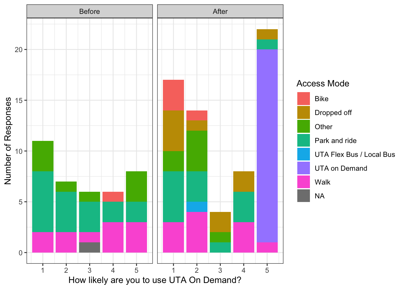
Figure 3.1: Reported likelihood of using microtransit by transit access mode.
The next consideration is whether the expressed or observed likeliness to use the microtransit service is related to the demographic characteristics of the respondents. Noting the low response rate to many of the demographic questions (see Table 3.1), it is not possible to construct a model that would predict the likeliness score as a function of these characteristics in combination. It is still valuable, however, to consider how the observed distribution of these characteristics differs between individuals who are or are not likely to use the service. These distributions are shown in Table 3.2, along with the result of a two-sided Fisher exact test of independence between the indicated characteristic distribution and the three-category likeliness response.
expected.table <- function(tab){
  pt <- prop.table(tab)

  m <- matrix(1, nrow = nrow(pt), ncol = ncol(pt))

  m1 <- sweep(m, MARGIN = 1, rowSums(pt), `*`)
  m2 <- sweep(m1, MARGIN = 2, colSums(pt), `*`)
  out <- m2 * sum(tab)
  rownames(out) <- rownames(tab)
  colnames(out) <- colnames(tab)
  out
}

fisher_tests <- tibble(
  variable = c("Smartphone", "Household size", "Auto availablity", "Income",
               "Age", "Weekly transit use"),
  sl_table = list(
    "smartphone" = table(survey_data$phone,   survey_data$likeliness_f),
    "size"       = table(survey_data$size_cat,survey_data$likeliness_f),
    "auto"       = table(survey_data$autos,   survey_data$likeliness_f),
    "income"     = table(survey_data$income,  survey_data$likeliness_f),
    "age"        = table(survey_data$age,     survey_data$likeliness_f),
    "frequency"  = table(survey_data$frequency_cat, survey_data$likeliness_f)
  )
) %>%
  mutate(
    prop = map(sl_table, prop.table),
    expected = map(sl_table, expected.table),
    diff = map2(sl_table, expected, `-`),
    fisher = map(sl_table, fisher.test),
    results = map(fisher, glance),
    n = map_int(sl_table, nrow)
  )  %>%
  unnest(cols = results)
group_names <- str_c(fisher_tests$variable, "; Fisher p-value: ",
round(fisher_tests$p.value, 4))
fisher_table <- do.call(rbind, fisher_tests$sl_table) %>%
as_tibble(rownames = NA) %>%
rownames_to_column("Demographic") %>%
mutate(group = rep(group_names, times = fisher_tests$n)) %>%
relocate(group)
kbl(fisher_table, caption = "Distribution of Rider Characteristics by Reported Likeliness",
booktabs = T) %>%
kable_styling() %>%
collapse_rows(1:2,row_group_label_position = "stack", latex_hline = 'none',
row_group_label_fonts = list(italic = TRUE, bold = FALSE))| group | Demographic | Not Likely | Neutral | Likely |
|---|---|---|---|---|
| Smartphone; Fisher p-value: 0.5633 | No | 2 | 1 | 1 |
| Yes | 41 | 8 | 30 | |
| Household size; Fisher p-value: 0.2068 | 1 | 2 | 0 | 2 |
| 2 | 8 | 0 | 1 | |
| 3 | 4 | 1 | 0 | |
| 4+ | 14 | 3 | 11 | |
| Auto availablity; Fisher p-value: 0.6593 | 0 | 1 | 0 | 3 |
| 1 | 22 | 3 | 10 | |
| 2 | 12 | 3 | 9 | |
| 3 | 7 | 1 | 5 | |
| 4+ | 3 | 2 | 3 | |
| Income; Fisher p-value: 0.6873 | Less than $44,999 | 4 | 1 | 3 |
| $45,000 to $100,000 | 10 | 2 | 5 | |
| Over $100,000 | 9 | 0 | 6 | |
| Age; Fisher p-value: 0.0036 | Under 18 | 1 | 2 | 0 |
| 18-24 | 7 | 2 | 9 | |
| 25-44 | 28 | 1 | 17 | |
| 45-64 | 7 | 5 | 3 | |
| Over 65 | 1 | 0 | 0 | |
| Weekly transit use; Fisher p-value: 0.2937 | One day or less frequently | 11 | 3 | 4 |
| Two to four days | 18 | 4 | 22 | |
| Five days or more | 20 | 3 | 18 |
Smartphone use appears to not be a contributing factor in the likeliness of using microtransit, as almost all respondents use a smartphone regardless of their reported likeliness. We also fail to reject the null hypothesis of independence between the likeliness to use microtransit and both auto availability and household income. The joint distribution of reported likeliness and household size suggests there could be some dependence, with members of smaller households more frequently expressing reluctance to use microtransit. This finding, if it could be verified, would be somewhat counter to the expectations of UTA. A Fisher test of independence between household size and expressed likeliness still fails to conclusively reject the null hypothesis but given the small sample size and counter-intuitive results, future investigation is warranted. This is particularly true given that automobile availability and household size go hand-in-hand: a household with more individuals, particularly driving-age individuals, will be more constrained in their driving behavior even with multiple household automobiles. Considering these two variables together will be important for future research but cannot be attempted here. There is also a suggestive relationship between transit use frequency and the responded willingness, with more frequent users having somewhat more willingness to use microtransit.
A clear statistical result is shown, however, between the reported willingness to use microtransit and the age of the respondent. This significant result persists when we recombine the age categories as well as discard neutral responses. Table 3.3 shows the differences between the observed values in the joint distribution of these two variables and the expected values based on the marginal distributions were the two variables to be completely independent. The largest differences occur in three noticeable places. First, individuals in the 18-24 years old category are more likely to express willingness to use microtransit. Second, individuals between 45 and 64 are more likely to express a neutral opinion than a positive or strictly unlikely one. Finally, individuals between 25 and 44 are – perhaps surprisingly – substantially more likely to express a negative opinion than a neutral one; these individuals are also modestly more likely than expected to express positive willingness to use transit.
kbl(fisher_tests$diff[[5]], digits = 4, booktabs = T,
    caption = "Difference of observed and expected frequencies for age and likeliness") %>%
kable_styling()| Not Likely | Neutral | Likely | |
|---|---|---|---|
| Under 18 | -0.5904 | 1.6386 | -1.0482 |
| 18-24 | -2.5422 | -0.1687 | 2.7108 |
| 25-44 | 3.6145 | -4.5422 | 0.9277 |
| 45-64 | -0.9518 | 3.1928 | -2.2410 |
| Over 65 | 0.4699 | -0.1205 | -0.3494 |