2 Study Methodology
2.1 System Description
In November 2019, the Utah Transit Authority (UTA) launched an on-demand microtransit service in the southern part of Salt Lake County. This region –– illustrated in Figure 2.1 –– has primarily low-density suburban development but also hosts stations for UTA’s extensive rail transit network: the FrontRunner commuter rail operates between Provo and Ogden via downtown Salt Lake City on 30 minute peak headways; and the Blue and Red TRAX light rail lines connect to downtown Salt Lake City, the University of Utah, and Salt Lake International Airport (via transfer) on 15 minute peak headways. There are existing fixed route and route deviation services in the region, as well as park and ride facilities at most rail stations. UTA launched the microtransit service in an effort to improve the quality of service for passengers in the region, expand the effective accessibility of the rail transit stations, and reduce transit operating costs by potentially eliminating or reallocating fixed-route bus lines.
knitr::include_graphics("images/via-map.png", auto_pdf = TRUE)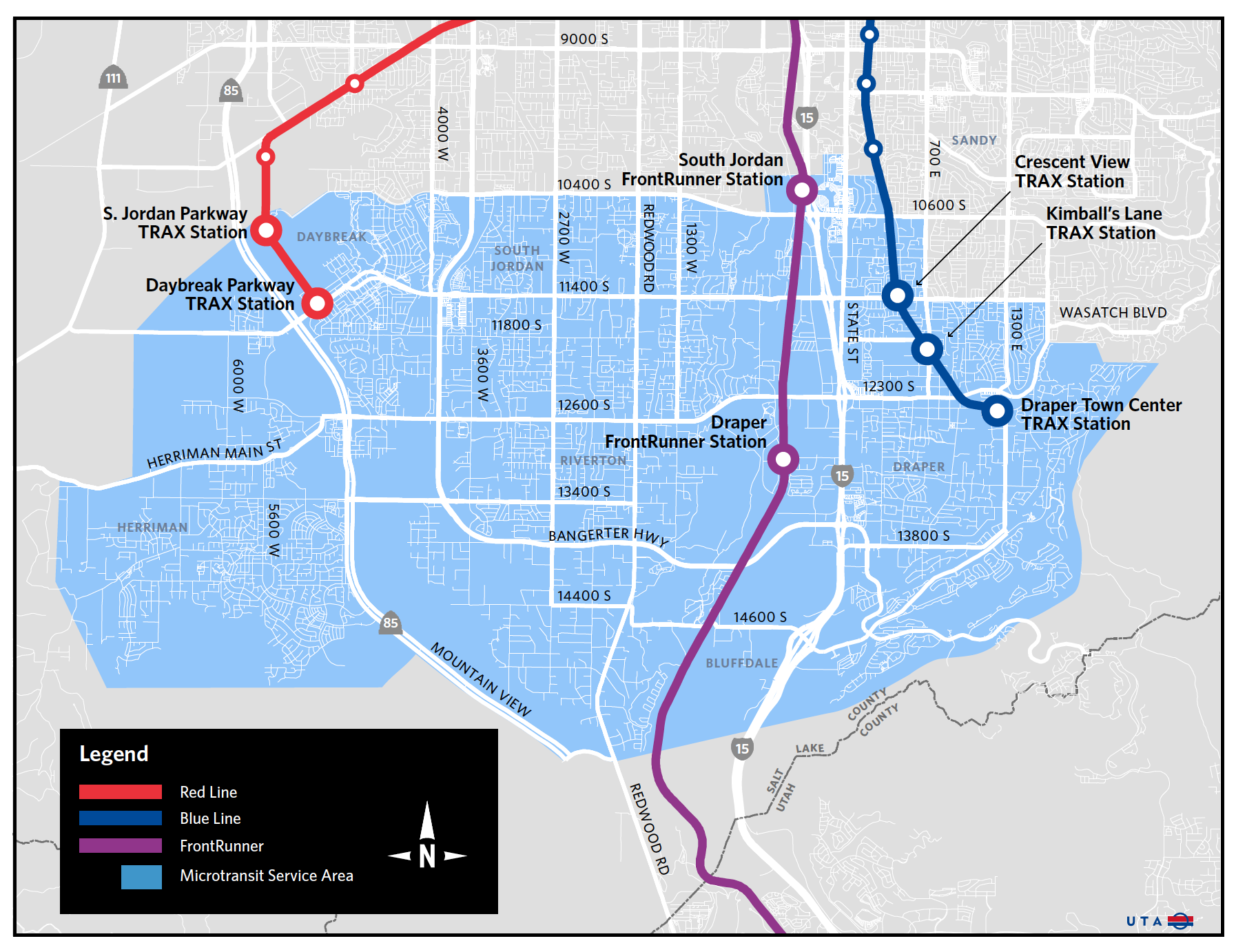
Figure 2.1: UTA on-demand microtransit service area. Image courtesy UTA.
In establishing the on-demand microtransit service UTA partnered with Via, a commercial mobility provider with new and ongoing operations in several US cities. Passengers request rides using the VIA mobile application or by calling a designated service line and await the vehicle at a pickup point near to their origin. Passengers share rides based on the availability of vehicles and the compatibility of paths, as determined by algorithms embedded in the VIA service. The vehicle will drop the passenger off near their destination or at TRAX or FrontRunner stations; both the pickup and drop-off points must lie within the service area shown in Figure 2.1. The regular adult one-way fare is $2.50 (the same as a regular base transit fare) and includes a limited transfer to the UTA fixed route transit system. By the end of February 2020, the microtransit system was carrying about 316 passenger trips per weekday with an average wait time of 11 minutes per trip (Utah Transit Authority 2020).
2.2 Survey Design
#' Function to read a qualtrics CSV file
#'
#' Qualtrics files are a little bit messy. This helps bring things
#' in with the right data types and descriptive column names
#'
read_qtrics_file <- function(file){
   headers <- read_csv(file, skip = 1, n_max = 0)
   csv <- read_csv(file, skip = 3, col_names = names(headers))

   namekey <- c(
     "Start Date" = "start",
     "How often do you ride UTA?" = "frequency",
     "Where are you headed today? - Selected Choice" = "purpose",
     "How did you travel to your UTA stop/station today? - Selected Choice" = "access",
     "Had you heard about UTA On Demand before today?" = "awareness",
     "How likely are you to download the VIA app and use UTA On Demand? - 1" = "likeliness",
     "Why did you choose that ranking?" = "likely_why",
     "What types of trips do you think you could use it for? - Selected Choice" = "use_purpose",
     "How many vehicles (cars, trucks or motorcycles) are available in your household?" = "autos",
     "Including YOU, how many people live in your household?" = "size",
     "What is your race / ethnicity? (check all that apply)" = "r",
     "Which of the following BEST describes your TOTAL ANNUAL HOUSEHOLD INCOME in 2019 before taxes?" = "income",
     "Do you have a smartphone?" = "phone",
     "What is your age?" = "age"
   )

   plyr::rename(
     csv,
     replace = namekey,
     warn_missing = FALSE
   )
}

# read files ==============
baseline <- read_qtrics_file("data/UTA+Baseline+Survey_July+21,+2020_16.23.zip")
q1_platform <- read_qtrics_file("data/UTA+January+Survey++-+Platform_March+16,+2020_14.07.zip")
q1_viastop  <- read_qtrics_file("data/UTA+January+Survey++-+VIA+Stop_March+16,+2020_14.07.zip")

# function to filter out the variables we care about
filter_data <- function(df){
  df %>% select(any_of(c(
   "start", "likeliness", "size", "autos", "income", "phone", "purpose",
   "frequency", "age", "access")))
}

get_period <- function(start){
  hour <- lubridate::hour(start)
  cut(hour, breaks = c(0, 6, 10, 15, 18, 24 ),
      labels = c("Night", "AM (6-10)", "Mid-Day (10-4)", "PM (4-7)", "Evening (7-Midnight)"))
}

# Bind tranches together and clean up
survey_data <- tibble(
  tranche = c("Before", "After", "After"),
  collection = c("baseline", "platform", "via stop"),
  data = list(baseline, q1_platform, q1_viastop)
)  %>%
  mutate( data = map(data, filter_data) ) %>%
  unnest(cols = data) %>%
  mutate(
    likeliness = ifelse(collection == "via stop", 5, likeliness),
    likeliness_f = factor(likeliness, labels = c(
      rep("Not Likely", 2), "Neutral", rep("Likely", 2))
    ),
    access = ifelse(collection == "via stop", "UTA on Demand", access),
    tranche = factor(tranche, levels = c("Before", "After")),
    period = get_period(start) ,
    income = case_when(
      income %in% c(
        "Less than $18,000", "$18,000 - $24,999", "$25,000 - $31,999",
        "$32,000 - $39,999", "$40,000 - $44,999") ~ "Less than \\$44,999",
      income %in% c(
         "$45,000 - $59,999",  "$60,000 - $74,999",  "$75,000 - $99,999") ~
        "\\$45,000 to \\$100,000",
      income %in% c(
        "$100,000 - $149,999", "$150,000 - $199,999", "$200,000 - $249,999",
        "$250,000 or above")  ~ "Over \\$100,000",
      TRUE ~ as.character(NA)
    ),
    income = factor(income, levels = c("Less than \\$44,999", "\\$45,000 to \\$100,000",
                                       "Over \\$100,000")),
    age = case_when(
      age %in% c("Under 16", "16-17") ~ "Under 18",
      age %in% c("18-24") ~ "18-24",
      age %in% c("25-34", "35-44") ~ "25-44",
      age %in% c("45-54", "55-64") ~ "45-64",
      age %in% c("65+") ~ "Over 65",
      TRUE ~ as.character(NA)
    ),
    age = factor(age, levels = c("Under 18", "18-24", "25-44", "45-64", "Over 65")),
    size_cat = factor(ifelse(size >= 4, '4+', size)),
    frequency_n = case_when(
      is.na(frequency) ~ as.numeric(NA),
      substr(frequency, 1, 1) %in% c("F", "N", "L") ~ 0,
      TRUE ~ as.numeric(substr(frequency, 1, 1))
    ),
    frequency_cat = case_when(
      frequency_n >= 5 ~ "Five days or more",
      frequency_n <= 1 ~ "One day or less frequently",
      TRUE ~ "Two to four days",
    ),
    frequency_cat = factor(frequency_cat, levels = c(
      "One day or less frequently", "Two to four days" , "Five days or more"))
  )
## Warning: Problem with `mutate()` input `frequency_n`.
## ℹ NAs introduced by coercion
## ℹ Input `frequency_n` is `case_when(...)`.## Warning in eval_tidy(pair$rhs, env = default_env): NAs introduced by coercionUTA’s primary goal in collecting a microtransit rider survey was to understand the effectiveness of its marketing campaign to raise awareness and information of the new service. This survey also provided an opportunity to inform additional riders and to evaluate rider perceptions and characteristics both before and immediately after the service launch. As such the survey was administered in two tranches. The first tranche was conducted on November 6th, 13th, and 14th of 2019 through on-platform intercept interviews at the Draper and South Jordan FrontRunner stations as well as the Draper Town Center TRAX station. The second tranche was collected on several weekdays between January 10th and March 4th, 2020, and was collected through on-platform intercept interviews at the same stations in addition to the Daybreak Parkway TRAX station and at designated microtransit pick-up points near the aforementioned rail stations. A limited number of interviews were also conducted on board the microtransit vehicles. Interviews were conducted throughout the day, but with a focus on the PM peak commute period; approximately 60% of the surveys in both tranches were collected between 4 and 7 PM.
The surveys were administered via electronic tablet using a questionnaire developed in a web-based survey software. The survey questions were developed with the help of UTA staff and an external consulting team. The relevant variables and source questions for this study are shown in Table 2.1, in the order in which the questions were asked. The interviewers approached subjects on the platform, identified themselves as conducting an informational survey on behalf of UTA, and informed the subjects that participation in the survey was anonymous and voluntary. After asking the respondent about their awareness of the system, the interviewer would give a brief explanation of the service before asking about the respondent’s likeliness to use the system. The questionnaire for the second tranche included additional questions that were identified as being important after the first tranche was collected; for example, the questions about income and household size were added between the tranches. Further, questions in the second tranche for respondents on train platforms and either at or on board the microtransit service had slightly different wording to reflect the separate contexts. There was also a set of questions requesting general feedback on the UTA service that is not included in this study.
questions <- tibble(
"Variable" =  c("Frequency", "Purpose",  "Access Mode", "Awareness",  "Likeliness",
                "Why Likely",  "Use Purpose", "Auto Availability",  "Household Size",
                "Race",  "Income", "Smartphone", "Age"),
"Question Text" = c(
  "How often do you ride UTA?",
  "Where are you headed today? ",
  "How did you travel to your UTA stop/station today?",
  "Had you heard about UTA On Demand before today? ",
  "How likely are you to download the VIA app and use UTA On Demand? ",
  "Why did you choose that ranking?",
  "What types of trips do you think you could use it for?",
  "How many vehicles (cars, trucks or motorcycles) are available in your household?",
  "Including you, how many people live in your household?",
  "What is your race / ethnicity?",
  "Which of the following BEST describes your TOTAL ANNUAL HOUSEHOLD INCOME in 2019 before taxes?",
  "Do you have a smartphone? ",
  "What is your age?"),
"Response Type" = c(
  'Multiple choice with days per week ',
  'Multiple choice with purposes plus text "other"',
  'Multiple choice with modes plus text "other" ',
  'Yes / No ',
  'Likert scale with five "likely" levels ',
  'Text response',
  'Multiple choice with purposes plus text "other"',
  'Multiple choice with 0 through 4+',
  'Multiple choice with 0 through 4+',
  'Mutiple choice allowing multiple selection ',
  'Multiple choice in ranges',
  'Yes / No ',
  'Multiple choice in ranges')
)

if(knitr::is_latex_output()){
  questions %>%
    kable(caption = "Survey Questionnaire Summary", booktabs = TRUE, format = "latex")  %>%
    kable_styling() %>%
    column_spec(2:3, latex_column_spec = "p{0.4\\\\textwidth}")
} else {
  questions %>%
    kable(caption = "Survey Questionnaire Summary")  %>%
    kable_styling()
}| Variable | Question Text | Response Type |
|---|---|---|
| Frequency | How often do you ride UTA? | Multiple choice with days per week |
| Purpose | Where are you headed today? | Multiple choice with purposes plus text “other” |
| Access Mode | How did you travel to your UTA stop/station today? | Multiple choice with modes plus text “other” |
| Awareness | Had you heard about UTA On Demand before today? | Yes / No |
| Likeliness | How likely are you to download the VIA app and use UTA On Demand? | Likert scale with five “likely” levels |
| Why Likely | Why did you choose that ranking? | Text response |
| Use Purpose | What types of trips do you think you could use it for? | Multiple choice with purposes plus text “other” |
| Auto Availability | How many vehicles (cars, trucks or motorcycles) are available in your household? | Multiple choice with 0 through 4+ |
| Household Size | Including you, how many people live in your household? | Multiple choice with 0 through 4+ |
| Race | What is your race / ethnicity? | Mutiple choice allowing multiple selection |
| Income | Which of the following BEST describes your TOTAL ANNUAL HOUSEHOLD INCOME in 2019 before taxes? | Multiple choice in ranges |
| Smartphone | Do you have a smartphone? | Yes / No |
| Age | What is your age? | Multiple choice in ranges |
To determine the significance of the relationship between the demographic characteristics presented in Table 2.1 and expressed willingness to use the on-demand microtransit service, we employ the Fisher “exact” test of independence in contingency tables (Fisher 1922). In this test the null hypothesis is that the two distributions are independent with the alternative being there is some dependence between the characteristic and the response. A \(p\)-value less than a given critical threshold indicates that the null hypothesis has a low probability and may be rejected. A conventional value of the critical value is \(\alpha=0.05\), though given the small sample sizes in this survey other critical values may be suggestive of the need for future evaluation. An attempt to use multiply-imputed datasets following the methodology of van Buuren and Groothuis-Oudshoorn (2011) and Licht (2010) was abandoned due to the missingness in the data, and the likelihood that the data were not missing at random (Jakobsen et al. 2017).