| Year | Principal | Interest | Loan Balance |
|---|---|---|---|
| 0 | 50000 | 0 | 50000 |
| 1 | 50000 | 5000 | 55000 |
| 2 | 50000 | 5000 | 60000 |
| 3 | 50000 | 5000 | 65000 |
| 4 | 50000 | 5000 | 70000 |
| 5 | 50000 | 5000 | 75000 |
4 Financial Project Evaluation
For which of you, intending to build a tower, sitteth not down first, and counteth the cost, whether he have sufficient to finish it? Lest haply, after he hath laid the foundation, and is not able to finish it, all that behold it begin to mock him, Saying, This man began to build, and was not able to finish. Luke 14
Infrastructure takes money to build. Money pays for the people to plan and build projects including tradesmen, construction managers, and engineers. Money also buys building supplies, construction equipment and land on which the project is to be built. How can you know if the money you spend on a project will be worth it? If you have many different options, how can you decide which one to build? How can you deal with the fact that money changes value over time?
Private businesses will evaluate a construction project as to whether it can return a reasonable profit. Governments may choose to build a project that provides the most benefits for their citizens at the lowest cost. Either way, a well-informed business, non-profit organization, or government will conduct a financial analysis of a potential construction project before committing to it. In addition, a financial analysis can guide planners, engineers, and construction managers on the appropriate design, scope, timeline, and resulting costs of an infrastructure project.
Think
Many of the principles and techniques you learn in this unit can apply to your own life, despite the meaningful differences between running a government or business and running a home. President Gordon B. Hinckley cautioned,
I recognize that it may be necessary to borrow to get a home, of course. But let us buy a home that we can afford and thus ease the payments which will constantly hang over our heads without mercy or respite for as long as 30 years. … I urge you, brethren, to look to the condition of your finances. I urge you to be modest in your expenditures; discipline yourselves in your purchases to avoid debt to the extent possible. Pay off debt as quickly as you can, and free yourselves from bondage.
Important
Many of the terms we use in this unit are used casually or differently by individuals, businesses, and industries (Boyte-White 2024). In this class, we will try to be consistent with our use of these terms. As a professional, it will be your responsibility to understand how each term is defined when evaluating financial analysis of a project or when communicating your results to others.
If you are unfamiliar with a term, look it up! Or ask! There are many good credible resources online. For example, see the Investopedia Dictionary (Investopedia 2024) and the U.S. Consumer Financial Protection Bureau glossary (US CFPB 2024a).
As always, you should know definitions for the terms in bold.
4.1 Returns and ROI
Learning Outcomes
- Calculate the returns for a single period project.
- Calculate return on investment (ROI) for a single period project.
- Discuss the benefits and risks of debt leveraging on ROI.
Whenever you have a financial project — this can be something as basic as a savings account or as complex and large as a multi-year heavy civil construction project — you hope that what you get out of the project will be worth at least as much as you put into it. After all, if you don’t get more money than you started with, why even do it? You might as well have put your money in a mattress.
What we put into a project is called its investment. What we get out of a project are called its returns. Mathematically, the returns are
\[ \mathrm{Returns} = \mathrm{Revenue} - \mathrm{Expenses} - \mathrm{Financing} - \mathrm{Taxes} + \mathrm{Sale\ value} - \mathrm{Capital\ investment} \tag{4.1}\]
Each of these terms in Equation 4.1 deserves a definition.
- Revenue is the money earned from operating the project.
- Expenses is money spent during a project in order to operate it. This might include supplies, wages, and equipment repairs.
- Financing are payments required by any loans associated with the project.
- Taxes are payments to the government required as part of a project’s operations or profits.
- Sale value is the money you make by selling the project, or could make by selling the project.
- Investment is the money you spend to acquire the project, or to permanently improve it.
We will cover taxes later in Section 4.6.
Any positive return is better than a loss, but a small positive return on a massive investment would be disappointing. We need a measure that can normalize how well a project does relative to its investment. A measure the effectiveness of an investment is return on investment or ROI. This is simply the ratio of returns to investments, or
\[ ROI=\frac{\mathrm{Returns}}{\mathrm{Capital\ investment}} \tag{4.2}\]
We often describe ROI as a percentage.
ROI and winning / losing
Note that the capital investment is counted twice in the ROI formula: once in the denominator, and once again in the returns equation (Equation 4.1). This leads to some interesting observations:
- A project with a 25% ROI means we grew our investment by 25%, which is in one year is much higher than the rate of inflation, or savings accounts, or even the average stock market. So this would probably be considered an excellent project. Even if you would be really disappointed to get 25% on an exam.
- A project with a 100% ROI means that we effectively doubled our investment.
- A project with a 0% ROI means that we didn’t make any money, but didn’t lose money either. Losing money would mean a negative return, and therefore a negative ROI.
Keeping the investment
What happens if you don’t sell the house at the end of the project?
When you make a capital investment you get to keep whatever you purchased, whether it’s a house or equipment or a piece of a company. Until you sell the investment you don’t know what its true value will be, but its value probably didn’t go to zero, and this value should be included in the project’s returns.
Maybe you have purchased an asset like stock in a company that always has a known value.
Returns on a stock
You purchased one share in the Caterpillar heavy equipment manufacturer in 2024 for $397. In October 2025, this stock was worth $500. What is your ROI?
Although you will not realize your returns until you sell the stock, you can still calculate a return on your investment to this point.
\[\begin{align*} \mathrm{Returns} &= \mathrm{Revenue} - \mathrm{Expenses} - \mathrm{Financing} - \mathrm{Taxes} + \mathrm{Sale\ value} - \mathrm{Capital\ investment}\\ &= 0 - 0 - 0 - 0 + 500 - 397\\ &= 103 \end{align*}\]
\[\begin{align*} ROI&=\frac{\mathrm{Return}}{\mathrm{Investment}}\\ &=\frac{103}{397}\\ &= 0.259 \end{align*}\]
Public company stocks always have a known market price. The value of things like real estate or stock in a private company might be more hazy, but until you realize the price you can at least assume that you didn’t lose value, or you can make a guess at what the value of the property might be.
Returns without a sale
You invest $480,000 to buy and rennovate a house in Provo. you think that these improvements increased the value of the home to at least $500,000.
Although in this case the $500,000 is just an estimate, you can still calculate a prospective return on your investment.
\[\begin{align*} \mathrm{Returns} &= \mathrm{Revenue} - \mathrm{Expenses} - \mathrm{Financing} - \mathrm{Taxes} + \mathrm{Sale\ value} - \mathrm{Capital\ investment}\\ &= 0 - 0 - 0 - 0 + 500000- (400,000 + 80,000)\\ &= 20,000 \end{align*}\]
\[\begin{align*} ROI&=\frac{\mathrm{Return}}{\mathrm{Investment}}\\ &=\frac{20,000}{480000}\\ &= 0.0417 \end{align*}\]
Of course, the question remains that if we thought the new value would be higher or lower, it might change whether we do the project in the first place.
For homework in this class, IF YOU ARE NOT TOLD WHAT THE NEW VALUE OF THE INVESTMENT IS, ASSUME IT DID NOT CHANGE.
Let’s explore the other parts of the Returns equation in Equation 4.1. If you have operating expenses or are collecting revenue from your project, you need to account for that in your calculations of the returns.
Capital investment or expense?
Expenses and investments in a project each reduce the returns in Equation 4.1, so why does it matter where you put them? When you are calculating the taxable income on your project (see Section 4.6), you can often deduct expenses, but you cannot usually deduct investments. Where you put investments and where you put expenses also affects the ROI. In the prior example, the cleanup is an expense of operating the project.
Investments involve permanent improvements, and expenses are general tasks required to maintain. Installing a new roof is an investment, fixing a leak in a roof is an expense. That doesn’t mean expenses can’t be expensive!
What happens when you use debt to start a project? This will decrease the returns from the project, because you will have to pay interest to the person who lent you the money. But you won’t have to invest as much in the project to start with, because that money isn’t yours. This can substantially increase the profitability of the project. We will cover the details of interest in Section 4.2, but we will consider what happens to the project ROI here.
This process of using debt to increase the profitability of a project is called leveraging. There are of course pros and cons associated using debt in this way. The returns go down, meaning that doing one project with debt would be a little less profitable than doing one project without it. But because you have less of your own resources invested in that one project, you could maybe do two projects! In that way you can increase your total overall returns across for the same amount of investment. That’s one reason why ROI is a good measure.
The cons of using debt to finance a project come when the project is unsuccessful. What if you don’t find renters? Or the repairs cost $50000? In that case, you don’t just lose your investment; the bank loses theirs also and you might not be able to borrow again on advantageous terms.
4.2 Time Value of Money
Learning Outcomes
- Describe why money in the future is worth less than money now.
- Calculate equivalent future and present values using simple and compound interest, with different compounding rates.
Imagine you win a contest and are given two options. You can choose to collect your $1,000 prize today, or you can wait for ten years to get the same amount of money. Which option would you choose? There are at least three reasons you should take the money right away:
- Risk There is a possibility that something bad could happen to your prize. Within the next 10 years, the company offering the prize could go bankrupt. Or you could die or become otherwise disqualified from claiming the prize.
- Inflation Money loses value over time for a variety of reasons. $1000 will buy more goods and services now than it will in ten years.
- Opportunity cost If you got the prize now, there are things you could do with it. You could spend the money on something that you would enjoy for the next ten years. You could also invest the money for ten years, during which time you would earn on that investment. Getting the prize later costs you these opportunities.
Money has value. Having money now is more valuable than having money in the future. This is called the time value of money. If I were to lend you money, I would want to receive not only the initial loan amount, but some payment to compensate me for the risk, inflation, and opportunity cost of making the loan. This payment is called interest. There are two basic methods for calculating interest:
- Simple interest loans require a defined interest payment on the principal of the loan, or how much the loan is for.
- Compound interest loans recompute interest along with the unpaid principal at a particular compounding rate.
If we have a simple interest loan, we can convert a present value of money \(P\) into a future value of money \(F\) with the formula: \[ F_\mathrm{simple}= P + P\times{i}\times{n} \tag{4.3}\] where \(i\) is the interest rate (usually percent per year) and \(n\) is the number of interest periods (usually years). In each year, we pay an interest charge \(P\times i\).
Warning
Interest rates are usually given in percentages (e.g., an interest rate of 12%), but should be used as decimal proportions in equations (e.g., \(i = 0.12\)).
While simple interest loans are easy to calculate and understand, almost all investments and loans use compound interest. The amount we will pay in the future \(F\) on a loan requires a little derivation. After one period, the compound interest formula looks just like the simple interest one, \[ F = P + P\times i=P(1+i) \tag{4.4}\] If we have two periods, then we need to take the value from Equation 4.4 and multiply it by \(i\), plus add another Equation 4.4 again for the new interest we add in year 1 \[ F = P(1+i)+P(1+i)i=P(1+i)(1+i)=P(1+i)^2 \tag{4.5}\]
If we keep doing this for \(n\) periods, we can derive a general equation \[ F = P(1+i)^n \tag{4.6}\]
One consideration with compound loans is the compounding frequency, or how often the interest is applied into the total amount owed. Usually, the compounding frequency and the interest rate and the number of periods will all be the same: that is, \(n\) will be in years and \(i\) will be in percent per year, with annual compounding.
But that might not always be the case! Sometimes loans could compound more frequently than once per year. Many mortgages, for example, give a nominal interest rate per year, but actually compound monthly. In this case, Equation 4.6 becomes
\[ F=P[1+(i/k)]^{nk} \tag{4.7}\]
with \(k\) the number of compounding periods in each \(n\). You can see how this works: the nominal interest rate is divided across \(k\) periods, but the total number of periods multiplied to \(nk\). \(i/k\) is referred to as the periodic interest rate.
Compounding frequency
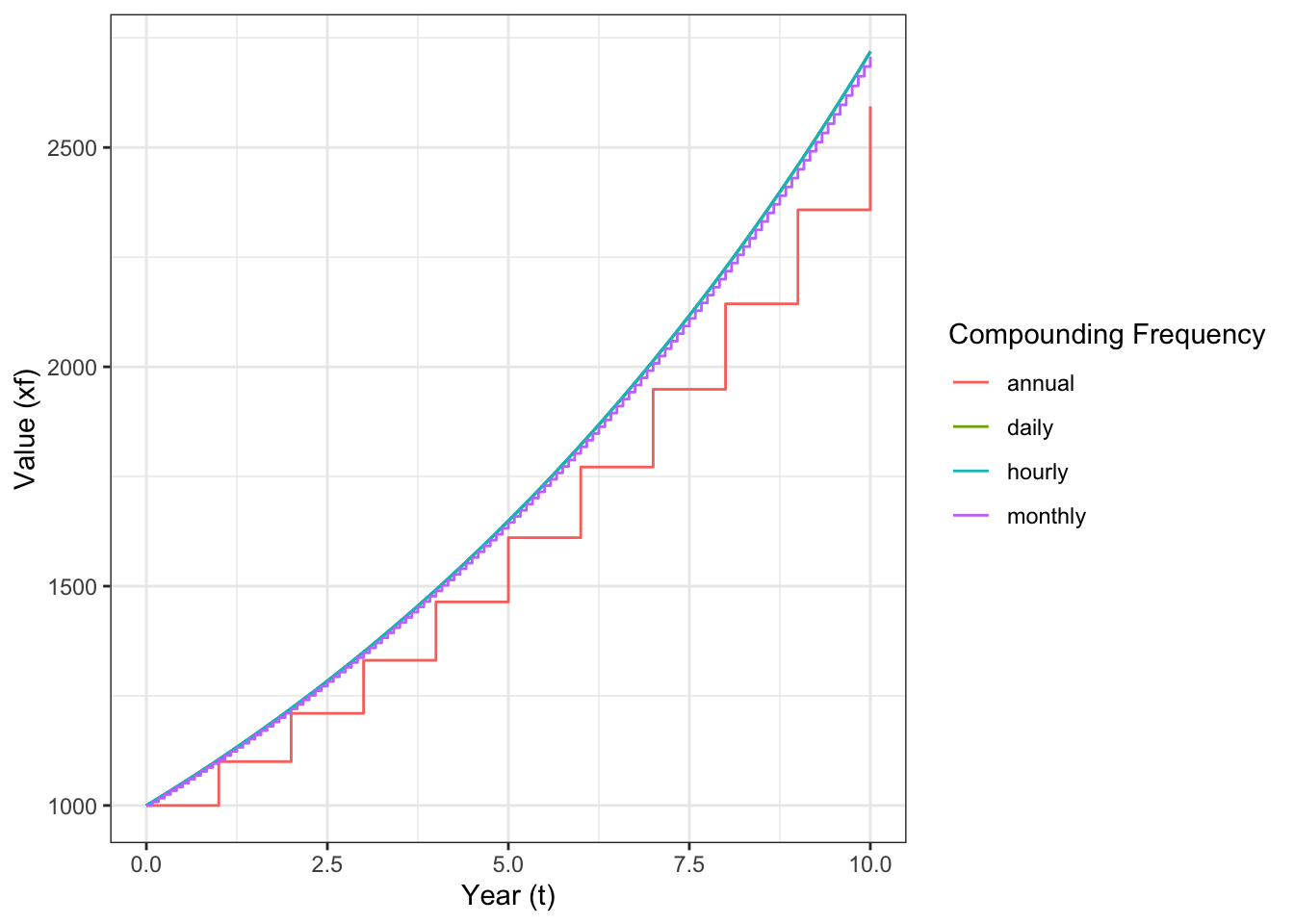
The compounding frequency has a pretty important role in how much the loan is worth in the future. Let’s look at three situations where $1000 is loaned at 10% interest (\(i = 0.1\)) for ten years.
- Yearly compounding (\(k\)=1): \(\$1000[1+(0.1/1)]^{(1*10)}=\$2593.74\)
- Monthly compounding (\(k\)=12): \(\$1000[1+(0.1/12)]^{(12*10)}=\$2707.04\)
- Daily compounding (\(k\)=365): \(\$1000[1+(0.1/365)]^{(365*10)}=\$2717.91\)
Figure 4.1 shows the growth in the loan amount at each compounding period for different compounding frequencies. There is obviously a big difference between annual and monthly compounding, but there isn’t that much difference between monthly and daily, or daily and even hourly compounding. This suggests that there is a limit to this function as \(k\) increases.
Continuous compounding
It turns out that if you take the limit \(\lim_{k\to\infty} F=P[1+(i/k)]^{nk}\) you can derive the equation for continuously compounding interest, \[ F=Pe^{in} \tag{4.8}\]
Using our new equation, we can find out how much money we will have after 10 years of continuously compounding the interest from our $1,000 invested at an interest rate of 10%.
- Continuously: \(\$1000*e^{(0.1*10)}=\$2718.28\)
Notice that this value isn’t significantly more than the amount of interest earned by compounding the interest daily. As the number of compounding periods continues to increase, the interest earned in each period increases by a diminishing amount. However, remember that even when the difference may be small, the more frequent the compounding period, the more interest is generated.
You may see bank advertising their savings accounts with an Annual Percentage Yield (APY) instead of an interest rate (Chen 2024). The APY is an annual interest rate compounded once per year that would give you the same returns as the actual or periodic interest rate using the compound frequency of the bank.
So after one year (\(n = 1\)), the future value of the investment over 1 year using the APY and the periodic interest rate and compounding frequency should be equal to each other:
\[\begin{align*} F_{\mathrm{annual}} &= F_{\mathrm{actual}} \\ P(1+APY)^n &= P(1+i/k)^{nk} \\ P(1+APY)^1 &= P(1+i/k)^{k*1} \end{align*}\] \[ APY = (1+i/k)^k -1 \tag{4.9}\]
The APY allows investors to compare returns from investments that have different compound periods.
Terms for \(i\)
Depending on the context of the problem, the term \(i\) may be described as an interest rate, a yield, or a discount rate. The term “discount” is used because when we calculate how much future money is worth in the present, we have to “discount” it for risk, opportunity cost, and inflation.
The term “inflation rate” is not generally appropriate for \(i\) on its own, because this would ignore the opportunity cost and risk aspects of the time value of money. But if you have no other options for investing and the risk is very low, then \(i\) and inflation rates can be very similar. During economic recessions the yield on US Treasury Bonds is often close to the inflation rate, because the US Government is seen as a low-risk investement, and other options in the economy are less attractive.
4.3 Annuities and Gradients
Learning Outcomes
- Calculate equivalent future and present values for uniformly repeating (annuity) and uniformly increasing (gradient) cash flows.
- Calculate equivalent values using equations, factor tables, and software functions.
In Section 4.2, you learned how to convert present values of money into future values of money and vice versa. But there are other ways of representing cash flows. Consider the following questions:
- How can I convert the present cost of a home into a monthly payment that I can afford over the next 30 years?
- If I have a piece of equipment that generates an income of $10,000 per year, what should I sell this equipment for now?
- If I want to buy a $400,000 crane for my business in five years, how much should I save each year?
All of these questions involve transforming a present value \(P\) or a future value \(F\) into an equivalent uniform value. Because the periods we use are often years, we often call this annual uniform value an annuity, \(A\).
Let’s do a short derivation to calculate the \(A\) needed to equal a future value \(F\). If there is only one period, then the derivation is easy and \(F = A\). If it takes two periods, then the equation is \(F = A + A*(1 + i)\) because we have to discount the value of the second period’s payment. If you do this for \(n\) periods (see the full derivation in the callout below), you get
\[ F = A*\frac{(1 + i)^n - 1}{i} \tag{4.10}\]
\(F = A\) derivation
Extending the full series \(n\) times gives you this summation.
\[\begin{align} F &= A + A*(1 + i) + A* (1 + i)^2 + \ldots + A*(i+1)^{n-1} \\ &= \sum_{j = 0}^{n -1} A ( 1 + i)^j\\ \end{align}\] If you multiply both sides of this equation by \((1 + i)\) this changes the index on the summation to have \(j\) start at 1 and go all the way to \(n\) \[\begin{align} F(1 + i) &= \sum_{j = 1}^n A ( 1 + i)^j \\ \end{align}\] Let’s subtract the equation for \(F= \sum_{j = 0}^{n -1} A ( 1 + i)^j\) from both sides of this new equation, which will allow us to subtract out everything except the first value of the first summation, and the last value of the second summation. We can then solve the equation for \(F\),
\[\begin{align} F(1 + i) - F &= \sum_{j = 1}^{n } A ( 1 + i)^j - \sum_{j = 0}^{n-1} A ( 1 + i)^j \\ &= \left[A ( 1 + i)^n + A ( 1 + i)^{n-1} + \ldots + A ( 1 + i)^1\right] - \\ &\quad \left[A ( 1 + i)^{n-1} + A ( 1 + i)^{n-2} + \ldots + A ( 1 + i)^0\right] \\ F+ Fi - F &= A*(1 + i)^n - A\\ Fi &= A*[(1 + i)^n - 1]\\ F &= A*\frac{(1 + i)^n - 1}{i} \end{align}\]
To turn a future value into an equivalent annuity, we just take the inverse.
\[ A=F*\frac{i}{(1+i)^{n}-1} \tag{4.11}\]
We could also derive an equation to convert a uniform repeating value into its present equivalent value P, but we will skip that derivation here because it’s very similar to the one we just did. The equation to convert \(A\) to \(P\) is:
\[ P=A*\frac{(1 + i)^n -1}{i (1 + i)^n} \tag{4.12}\] and for \(P\) to \(A\):
And from \(P\) to \(A\) is of course the inverse of that: \[ A=P*\frac{i ( 1 + i) ^n}{(1 + i)^n - 1} \tag{4.13}\]
This last Equation 4.13 is the equation that a bank will use to figure out what the monthly or annual payment is for a loan with a periodic pay back period. In this case the principal of the loan is the present value \(P\), and you need to repay the loan with an equivalent uniform payment \(A\).
As in Equation 4.7, we can convert nominal discount rates given in percent per year to use different compounding periods by dividing \(i/k\) and \(n*k\). This is pretty common, because many loans for things like cars and homes are repaid with monthly compounding interest and monthly payments.
In most of our equivalence functions we have looked at, we assume some project end-point \(n\) time periods in the future. But what about the equivalent present value of a perpetual benefit? Like, what if a project that generates annual uniform benefits \(A\) is meant to last forever?
Consider Equation 4.12, as \(n\) gets really big
\[\begin{align*} P&=A*\frac{(1 + i)^n -1}{i (1 + i)^n}\\ &=A*\frac{(1 + i)^\infty -1}{i (1 + i)^\infty}\\ &=a*\frac{1}{i}\frac{(1 + i)^\infty -1}{(1 + i)^\infty}\\ &=a*\frac{1}{i}\frac{\infty - 1}{\infty}\\ \end{align*}\]
Because \(\infty-1 \approxeq \infty\), and \(\infty/\infty = 1\), this equation reduces to a simple long-run equation,
\[ P=\frac{A}{i} \tag{4.14}\]
It turns out that it doesn’t even have to infinite timelines to get to this point. With high values of \(i\) (like 15%), this simplification is reasonably accurate in as little as 25 years.
4.3.1 Gradients
We have talked about repeating uniform value?. But what about a payment or cost that increases its value over time by a uniform amount? For instance, you expect that maintenance costs on a machine will increase each year, or you expect that a business line will grow, bringing in more revenue.
A uniformly increasing money flow is called a gradient, and we will represent this with the letter \(G\)[^financial-4]. Uniformly increasing means that if \(G = 100\), then the value of this gradient in year 1 is 0, but it increases by 100 in each subsequent year as \(G_1 = 0, G_2 = 100, G_3 = 200, \ldots, G_n = (n-1)*G\).
The formulas to convert a uniform increasing value \(G\) to a present value \(P\), a future value \(F\), or a uniform value \(A\) are:
\[ P=G*\left[\frac{(1+i)^{n}-1}{i^2(1+i)^{n}}-\frac{n}{i(1 + i)^n}\right] \tag{4.15}\]
\[ F=G*\left[\frac{(1+i)^{n}-1}{i^2}-\frac{n}{i}\right] \tag{4.16}\]
\[ A=G*\left[\frac{1}{i}-\frac{n}{(1+i)^n-1}\right] \tag{4.17}\]
Example
Maintenance on an old machine is $100 this year but is expected to increase by $25 each year thereafter. What is the present worth of five years of maintenance? Assume a discount rate of 10%.
This is an interesting problem because it involves both an annuity ($100 per year) and a gradient of $25 each year. We could draw a diagram of these cash flows as
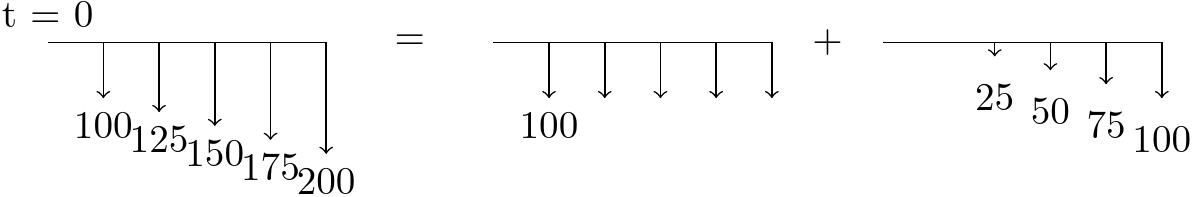
We can then calculate the present value of each element separately and add them together. Converting the gradient \(G = 25\) to its present value, \[\begin{align*} P&=G*\left[\frac{(1+i)^{n}-1}{i^2(1+i)^{n}}-\frac{n}{i(1+i)^{n}}\right]\\ &=25*\left[\frac{(1+0.1)^{5}-1}{(0.1)^2(1+0.1)^{5}}-\frac{5}{0.1(1+0.1)^{5}}\right]\\ &=172\\ \end{align*}\]
and converting the annuity \(A = 100\) to its present value, \[\begin{align*} P&=A*\frac{(1+i)^{n}-1}{i(1+i)^{n}}\\ &=100*\frac{(1+0.1)^{5}-1}{0.1(1+0.1)^{5}}\\ &=379 \end{align*}\]
meaning that we have a total present value of $551
4.3.2 Calculation Shortcuts
It is important to know that the equations we have discussed so far exist, and that they are not magical constructs banks designed to part you from your money. But the equations themselves are often unwieldy and impractical, and they are certainly difficult to remember.
Notice though that each equation we have looked at is the product of a scalar (\(A\), \(F\), etc.) and some factor of the interest rate and the time period. This means we could create a table that contains the factors for different interest rates and periods. A partial table for 2% discount rates is in Table 4.3, and a complete set of tables are in Appendix A. The way to read these tables is as follows:
- Identify the table for the discount rate you are given.
- Determine which column of factors you need. You read \(F/P\) as “\(F\) given \(P\)”, so this is your column if you have been given a present value and wish to find the future value.1
- Find the row in the table for the given number of periods. If \(F/P\) is your column and the number of time increments is 5, your value is 1.1041.
- Multiply the given value by the factor from the table. Keeping with the same example, if you were given 1,000 dollars for \(P\), you multiply it by 1.1041 to find \(F\) = 1,104.10 dollars.
| n | P/F | P/A | P/G | F/P | F/A | A/P | A/F | A/G |
|---|---|---|---|---|---|---|---|---|
| 1 | 0.9804 | 0.9804 | 0.0000 | 1.0200 | 1.0000 | 1.0200 | 1.0000 | 0.0000 |
| 2 | 0.9612 | 1.9416 | 0.9612 | 1.0404 | 2.0200 | 0.5150 | 0.4950 | 0.4950 |
| 5 | 0.9057 | 4.7135 | 9.2403 | 1.1041 | 5.2040 | 0.2122 | 0.1922 | 1.9604 |
| 8 | 0.8535 | 7.3255 | 24.8779 | 1.1717 | 8.5830 | 0.1365 | 0.1165 | 3.3961 |
| 10 | 0.8203 | 8.9826 | 38.9551 | 1.2190 | 10.9497 | 0.1113 | 0.0913 | 4.3367 |
| 25 | 0.6095 | 19.5235 | 214.2592 | 1.6406 | 32.0303 | 0.0512 | 0.0312 | 10.9745 |
| 50 | 0.3715 | 31.4236 | 642.3606 | 2.6916 | 84.5794 | 0.0318 | 0.0118 | 20.4420 |
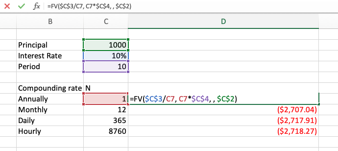
The factor table method is easy and helps to train you to think about what is happening. But it is slow when you have repeated calculations, which is common for large projects. In practice, you will probably use functions that pre-exist in Excel, Google Sheets, or another software application. For example, the Excel FV() function will compute the future value \(F\) of a cash flow given either an present value \(P\) or a uniform flow \(A\).
FV(rate, number_of_periods, payment_amount (A), [present_value (P)])If you are going to give a present value and not an annuity, you leave the payment_amount field blank. That means, the FV function works both as Equation 4.6 and also as Equation 4.10. The results and use of this function are shown in Figure 4.2. Table 4.4 provides a lookup table correlating the factor tables in Table 4.3 with the Excel and Google Sheets function equivalents.
| Factor | Excel / Sheets Function |
|---|---|
| P/F | PV(i, n, ,F) |
| P/A | PV(i, n, A) |
| P/G | Not included |
| F/P | FV(i, n, , P) |
| F/A | FV(i, n, A) |
| A/P | PMT(i, n, P) |
| A/F | PMT(i, n, , F) |
| A/G | Not included |
Custom functions
Sometimes you need to do an analyis that neither Excel nor the factor tables are well-suited for. Or, you might realize that Excel is poorly suited to most serious work. In this case, you may want to write your own functions in the software environment that you prefer. For example, we can write an R function for Equation 4.7 that converts \(P\) to \(F\), and then use that function to compute the future value for a strange loan that compounds 20 times per year.
#' Function to change P to F
#' @param P Present value
#' @param i Discount rate
#' @param n Number of periods
#' @param k Compounding iterations per period, default is 1
#'
#' @return Future value F
ptof <- function(P, i, n, k = 1){
  P * (1 + (i / k) )^(n * k)
}

# 1000 for ten years at 7.5%, compounding 20 times per year
ptof(P = 1000, i = 0.075, n = 10, k = 20)
[1] 2114.032The python code for the same function is here:
def ptof(P, i, n, k=1):
  """
  Function to convert P to F

  Parameters
  ----------
  P : float
      Present value
  i : float
      discount rate per period
  n : int
      number of periods
  k : int
      number of compounding events per period

  Returns:
    float: The future value of the money flow.
  """
  P * (1 + (i / k) )^(n * k)
Which method should I use?
For short homework problems and exam questions, we strongly recommend that you use factor tables. Write out what you are trying to find, what you have, and the factor you need to convert one to the other. So, if you are given an annuity \(A\) and need to find a present value \(P\), write out \[ P = A * P/A(i, n) \] and look up the appropriate factor.
For long homework problems where you may have to construct a spreadsheet with dozens of calculations, you should use the spreadsheet functions available to you.
You won’t have to write your own R or python functions in this class, but knowing that you can might be useful later in your career.
4.4 Net Present Value
Learning Outcomes
- Calculate the net present value (NPV) of a complex cash flow.
- Draw a cash flow diagram for a project.
In Section 4.2 and Section 4.3, we discussed how to calculate the present value of a cash flow, whether that flow was a single future value (\(F\)), a series of uniform values (\(A\)), or uniformly increasing (\(G\)) future values.
This is powerful because it allows us to translate complex cash flows defined with different interest rates and time frames into an equivalent present value. Recall the returns equation we developed back in Equation 4.1, but now let’s look at it with multiple years so that we can accommodate the time value of money.
As we have talked previously, the reason to invest in a projects is to receive a return of benefits. If you are a developer, you want to build something that will generate income justifying the cost of construction. If you are building public infrastructure, the benefits might not be economic (although they could be). We will now consider definition of returns that considers the time value of money.
To do so, we need to be more precise about the timing of the returns. We will use the definition of returns in Equation 4.1, but with a wrinkle to spread the returns across multiple years.
\[ \mathrm{Returns}_t = \mathrm{Revenue}_t - \mathrm{Expenses}_t - \mathrm{Financing}_t - \mathrm{Taxes}_t + \mathrm{Sale\ value}_t - \mathrm{Capital\ investment}_t \tag{4.18}\]
Where
- \(t\) is the years of analysis
- Revenue is the money earned from operating the project in the year \(t\).
- Expenses is money spent during a project in order to operate it in the year \(t\). This might include supplies, wages, and repairs.
- Financing are payments required by any loans associated with the project in the year \(t\).
- Taxes are payments to the government required as part of a project’s operations or profits.
- Sale value is the money you make by selling the project’s assets in the year \(t\). If you still own an asset at the end of the project, you would use the value you could make by selling the the asset, but only in the final year.
- Investment is the money you spend to acquire the project, or to permanently improve it, in the year \(t\).
When Equation 4.18 is calculated over the lifetime of the project, we obtain the earlier Equation 4.1. But that equation doesn’t consider that the positive returns at the end of a project are worth less than returns at the beginning, because of the time value of money.
Once you have the annual project returns, you need to bring those returns into the present so that you can compare earnings on an equal footing. The total value of all project returns in present worth is called the Net Present Value of the project. If the NPV is positive, then the project will result in a positive return on investment. If it is negative, then the project will lose money over its life. The equation for the NPV is just the sum of each year’s returns, converted to a present value using a discount rate, \[ NPV=\sum_{t=0}^{n} \frac{R_t}{(1+i)^t} \tag{4.19}\]
where
- \(R_t\): net returns at time \(t\)
- \(i\): discount rate
- \(t\): period of time
Note that the \(1/(1+i)^t\) is the same as Equation 4.6, or the equivalence function to bring a future value to the present.
It turns out it doesn’t really matter whether we first compute the net returns in each year and then transform these into present values, or if we first transform into present values and then add them up. The first method works better for complex projects, but the second might make more sense for simpler projects.
Note how in house flipping example, the bank issued a loan at an interest rate of 6%, but the NPV used a discount rate of 8%. This brings up the question of what discount rate should be used in NPV calculations, and how this discount rate is determined. Recall that the discount rate has to account for:
- Risk: when you lend money, it might not always come back
- Inflation: money will be worth less in the future
- Opportunity Cost: you might be able to do something else with your money
Different people and organizations have different time values of money based on their priorities, standards, and perceptions of the world. For example, investors will expect higher returns on more risky investments, and larger investors might not want to take on smaller projects. Either way, they will use a higher discount rate in their analysis. The disount rate that a company uses in its NPV analysis is called its Minimum Acceptable Rate of Return.
Setting the MARR
When a company is considering the MARR for its own projects, it considers the cost of raising capital. What this means is that the company can raise money for its projects by selling stock in itself on the market. If the return on the investment for doing a project is less than what the company would get by simply selling its own stock, the company will lose money relative to that baseline.
The cost of capital when it is a combined sources of capital is called the weighted average cost of capital (WACC). The WACC is calculated as (Blank and Tarquin 2023a):
\[ \mathrm{WACC}= (\mathrm{equity\ fraction})\times{(\mathrm{cost\ of\ equity\ capital})}+ (\mathrm{debt\ fraction})\times{(\mathrm{cost\ of\ debt\ capital})}\\ \tag{4.20}\]
Where the cost of debt capital is the interest rate on the debt. The cost of the equity is the expected rate of return of its company shares. By selling the shares, the company will not realized those returns, in other words, the equity costs is the opportunity cost of choosing to sell their equity.
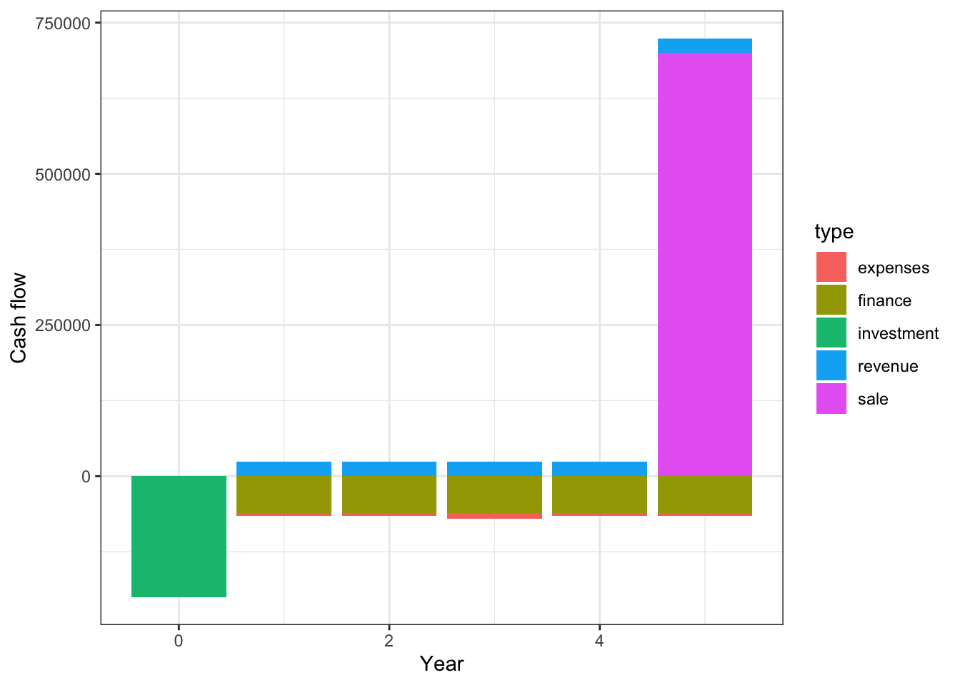
When you are doing NPV analysis on a complex cash flow, it is really useful to have a mechanism for understanding what is happening in each year. A cash flow diagram is simply a chart of the cash flows in each year of a project. Draw a negative bar for cash outlays (expenses, financing, etc.) and a positive bar for cash inflows (revenues, sale, etc.).
Note that you can draw this cash flow diagram for each type of cash flow, or as the net.
Multiple-year cash flow diagram
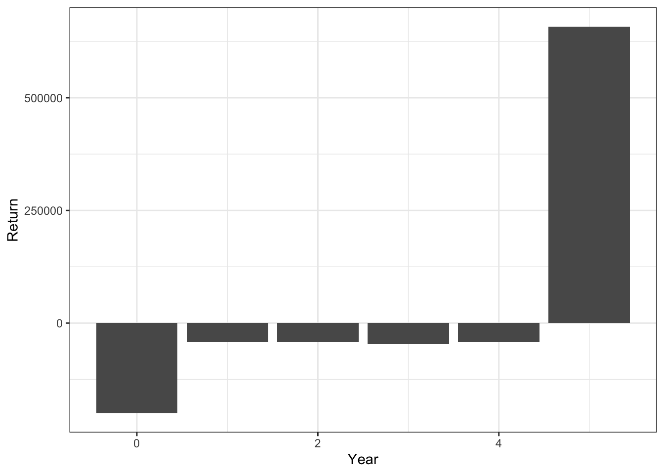
Draw cash flow diagrams for the Provo house-flipping project; include both a diagram of each element of the annual returns, and a diagram of the net returns in each year.
The charts below show these diagrams.
Solving NPV problems
Steps to solving NPV problems:
- Carefully read the problem, and identify what numbers are used for which variables. Is it an \(A\) or an \(F\)? Or an \(n\).
- Draw a cash flow diagram, which might help you discover any errors in step 1.
- Write out an equation for the NPV, using appropriate factors.
- Look up the factors and calculate a solution.
Appendix B includes a web application that will generate random cash flows, letting you practice solving NPV problems.
4.5 Internal Rate of Return
Learning Outcomes
- Calculate the internal rate of return for a complex cash flow.
In Equation 4.2 we looked at how to compute the return on investment for an investement that treats all expenses and earnings as if they occur in the same year. But most built environment projects are not one-year investments. Often, people will build expensive infrastructure hoping to earn revenues over many years. But the dollars earned as revenue late in a project are not the worth the same as the dollars invested early in the project. It would be nice to know the average return on investment on a project is when the costs and revenues occur in different years.
Consider a simple project with only a present investment value \(P\) and future returns value \(F\), as in Equation 4.6. The net present value of this project is \(NPV = -P + F*P/F(i, n)\). Let’s solve this equation for the discount rate \(i\) when the NPV is zero: \[\begin{align} NPV &= -P + F*P/F(i, n) \\ 0 &= -P + \frac{F}{(1 + i)^n} \\ P &= \frac{F}{(1 + i)^n} \\ \frac{F}{P} &= ( 1 + i)^n \\ \left(\frac{F}{P}\right)^{1/n} &= (1+i) \end{align}\] which reduces to \[ i = \left(\frac{F}{P}\right)^{1/n} - 1 \tag{4.21}\]
So, there is one particular value of \(i\) that effectively sets the future returns equal to the present investment value, with \((F/P)^{-n} - 1\). This is is called the Internal Rate of Return, or the IRR. The IRR of an investment is defined as the interest rate that makes the net present value zero. Or put another way, it is the interest rate at which all future earnings are equal to the investment.
Why is this value a rate of return, or a measure of return at all? Conceptually, it shows how much our initial investment grew over the course of our project, just like ROI is supposed to. But it works mathematically as well. We can add \(P/P\) and substract \(P/P\) (effectively adding 0) inside the parentheses, \[\begin{align} i&= \left(\frac{F}{P} - \frac{P}{P}+\frac{P}{P}\right)^{1/n} - 1 \\ &= \left(\frac{F-P}{P}+1 \right)^{1/n} - 1 \\ \end{align}\] Now, let’s consider that our traditional ROI equation in Equation 4.2 can be redefined as \(ROI = \frac{F-P}{P}\) with the returns from our investment divided over the amount of the investment. This the value we have inside our rearranged Equation 4.6! \[ i= \left(ROI +1 \right)^{1/n} - 1 \tag{4.22}\] Effectively, \(i\) in this case is an annualized ROI (Beattie 2024), with each year’s returns adjusted for inflation, risk, and opportunity cost.
IRR
You invest \(P\) into a savings account which yields a future value \(F\) after \(n\) years. The interest rate, \(i\), on the savings account is compounded yearly. Which of the following terms best describes \(i\)?
- Interest rate
- APY
- Internal rate of return
This is a tricky question. In this simple case \(i\) can correctly be defined by each of the terms. All of these values are the same in definition. However, only IRR is available when the cash flows get complex. Please note that sometimes the IRR is also referred to as the rate of return or the ROI. For exams, and in this textbook, we will refer to the IRR as the IRR. The ROI will be used to refer to return on investment without discounting future cash flows.
The benefit of IRR is that once we have calculated the NPV of a project — no matter how complex its costs and earnings — we now have a tool to immediately calculate the implied return from this project, and we don’t have to even know what the interest rate is, because it’s something we calculate in the problem. That’s worth noting again: the NPV requires an assumed discount rate, but the IRR does not.
For example, what if you make an investment \(P\), in order to receive an annuity of \(A\) over the next \(n\) years. What is the rate of return of your investment? We can use Equation 4.12 \[\begin{align*} P &= A*\frac{(1 + i)^n -1}{i (1 + i)^n} \end{align*}\] Unfortunately, Equation 4.12 is too complex to re-arrange to solve for \(i\) by algebra. Fortunately, there is another way to solve for \(i\). We can construct the net present value of this cash flow, \[ NPV = -P + A * P/A(i, n) \] and find the interest rate that sets \(NPV = 0\). We can do this by brute force — trying values until we get the right one — or by using optimization software included in spreadsheets or other programs.
IRR Example with Factor Tables
Margot decides to pursue a PhD degree in Civil Engineering while she is working. She pays upfront $30,000 for her tuition and books at the start of her program. She then earns an additional $5,000 per year for the next 5 years while a research assistant.2 In year 5, she successfully led a team to design an earthquake resistant bridge that was a direct outcome of her thesis. The President of her engineering firm gives her a bonus of $14,746.84. What is the IRR of her doctoral investment after 5 years? Is it 6%, 8%, or 10%?
To solve for IRR, we need to find the interest rate, \(i\) that yields an NPV = 0. Let’s draw a cash flow diagram of this problem to help us set up the NPV equation.
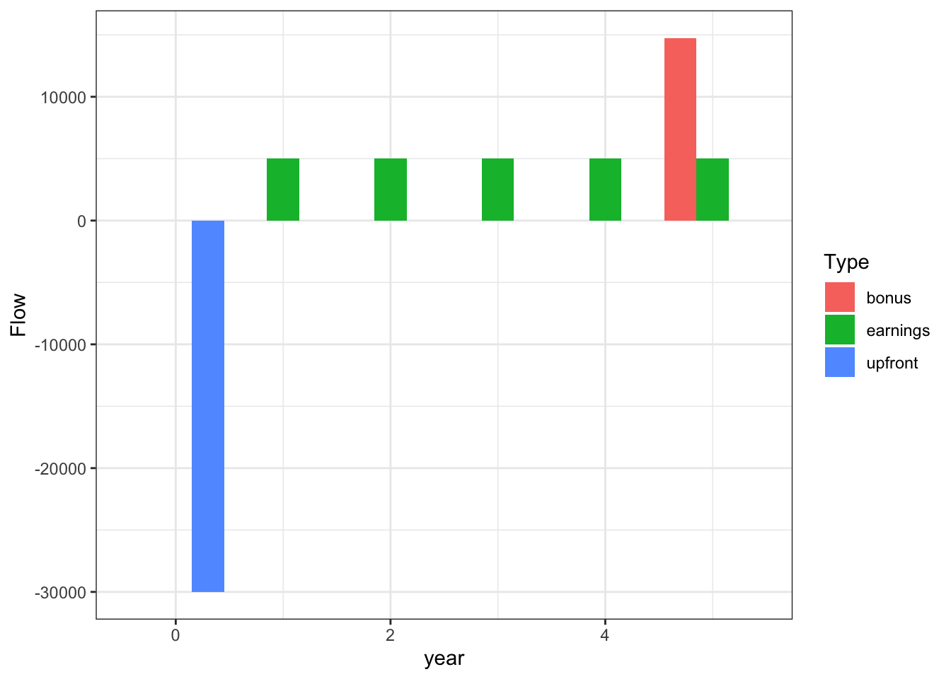
The upfront tuition and books are a present value \(P\), the RA wages are an annuity \(A\), and the bonus she gets is a future value \(F\). So the NPV equation we need to solve is
\[0 = P + A *P/A(5, i) + F * P/F(5, i)\]
Brute force method
Let’s set up a table that will calculate this equation for different values of \(i\). The final column, NPV is the equation above using the factors on that row. You can see that with a discount rate of 8%, the NPV is effectively zero, meaning that the IRR is very close to 8%.
| i | P | A | A/P | FV | F/P | NPV |
|---|---|---|---|---|---|---|
| 0.06 | -30000 | 5000 | 4.2124 | 14746.84 | 0.7473 | 2081.5156 |
| 0.08 | -30000 | 5000 | 3.9927 | 14746.84 | 0.6806 | 0.0017 |
| 0.10 | -30000 | 5000 | 3.7908 | 14746.84 | 0.6209 | -1889.4387 |
Graphical solution
We could use a graphing calculator to solve this problem by finding the point where the NPV function with respect to the interest rate is zero.
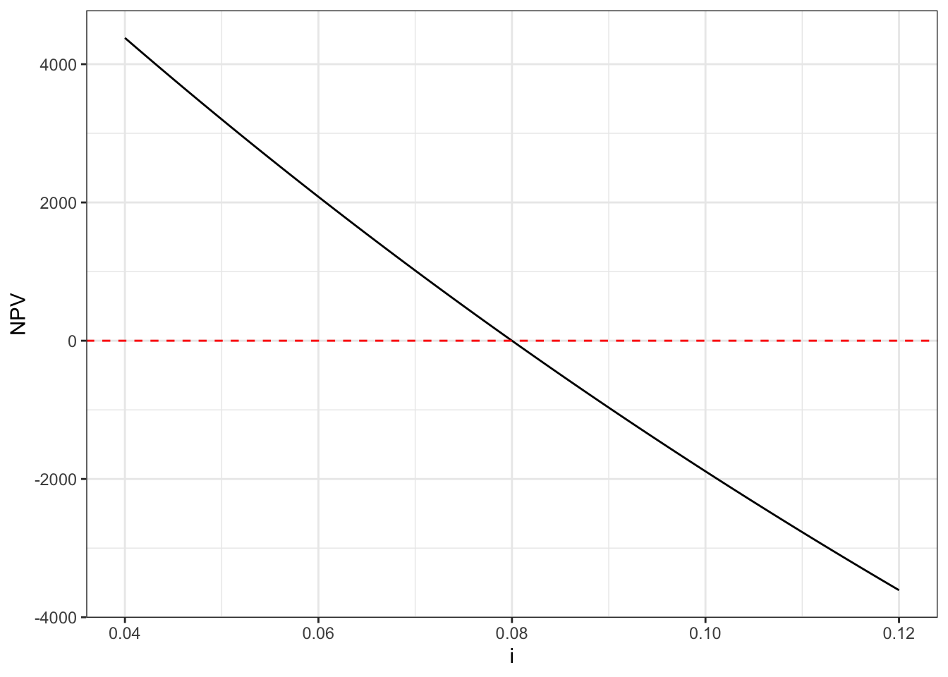
Because the line crosses at \(i = 0.08\), the IRR is close to 8%.
Excel goal seek
We can get a more precise measure of the IRR by using a numerical solution like Goal seek in Excel. Here is a video showing how to solve the problem with goal seek:
Numerical solver
Goal seek is not the only numerical solver. In this case, I can use the R optim function which works like goal seek.
# calculate NPV for different values of i
irr_example_fn <- function(i){
  NPV <- -30000 + atop(5000, i, 5) + ftop(14746.84, i, 5)
  abs(NPV) # find smallest NPV, positive or negative
}
# find value of i that makes this function 0, within bounds
o <- optim(0.06, irr_example_fn, method = "Brent", lower = 0, upper = 1)
o$par # This is the value of i that makes NPV 0
[1] 0.08000002Sure is close to 8%.
IRR limitations
There are situations with complex cash flows where the IRR is not unique; e.g., a complicated cash flow where costs and revenues occur in different times might result in zero NPV at 2% and at 9%. You can find these cases by plotting the IRR against the NPV and seeing if there are multiple points where the NPV is zero. In this case, you must use an alternative method to determine your project’s actual returns. Options may include an external rate of return, or a modified internal rate of return, or even just the NPV directly with a properly chosen discount rate.
Solving IRR problems
Steps to solving IRR problems:
- Carefully read the problem, and identify what numbers are used for which variables. Is it an \(A\) or an \(F\)? Or an \(n\)?
- Draw a cash flow diagram, which might help you discover any errors in step 1.
- Write out an equation for the NPV, using appropriate factors.
- Look up the factors and calculate the NPV. If your NPV is non-zero, repeat step 4 with a different discount rate.
Appendix B includes a web application that will generate random cash flows, letting you practice solving NPV and IRR problems.
4.6 Taxes
Learning Outcomes
- Calculate the taxable income for a project in a given year.
- Calculate depreciation of capital assets using straight-line and declining balance methods.
Taxes are “required payments of money to governments, which use the funds to provide public goods and services for the benefit of the community as a whole.” (US CFPB 2024b). In the private sector, you need to account for tax payments when you consider the profitability of your projects. In the public sector, taxes provide funding and incentivize the behavior of private sector actors.
Use accountants!
As a built environment professional, you should rely on certified accountants to understand the details of the tax code, provide advice on financial decisions, and/or file your taxes.
However, having a basic understanding of taxes and depreciation will help you make wise business and infrastructure investment decisions.
The tax a company pays in a year \(t\) is the product of its taxable income for that year and an applicable tax rate, \[ \mathrm{Taxes_t}=\mathrm{Taxable\ Income}_t \times \mathrm{Tax\ Rate} \tag{4.23}\]
Effective tax rates
In the US, most companies are required to pay both state and federal taxes. Federal tax code generally allows state taxes to be deducted from federal taxes. The effective tax rate a company pays combines both of these rates into a single number,
\[ \mathrm{Effective\ Tax\ Rate}=\mathrm{State\ rate}+(1-\mathrm{State\ rate})\times(\mathrm{Federal\ rate}) \tag{4.24}\]
In this class, you should assume that tax rates given in problems are effective tax rates unless told explicitly otherwise. Common corporate effective tax rates are on the order of 25% to 40%, depending on industry and state.
Taxable income for a given year \(t\) is defined as
\[ \mathrm{Taxable Income}_t = \mathrm{Revenue}_t - \mathrm{Expenses}_t - \mathrm{Interest}_t + \mathrm{Capital\ gains}_t - \mathrm{Depreciation}_t \tag{4.25}\]
Where
- Revenue is the money earned from operating the project.
- Expenses is money spent during a project in order to operate it. This might include supplies, wages, and equipment repairs.
- Interest are payments to repay the loans or debts of the project.
- Capital gains is money earned by selling capital assets.
- Depreciation is the loss of value in capital assets.
Note how similar Equation 4.25 is to Equation 4.1: taxable income is meant to be based on the returns of your project. There are three key differences, all related to the concept of capital assets. The basic principle of these differences is that you should be taxed for any growth in value, but that you should be able to deduct loss in value.
- When calculating returns in Equation 4.1, you consider the entire payment made to the bank as a “Financing” payment. In Equation 4.25, only the interest payments are deducted from taxable income. Money you pay on the principal is technically converted into value of the capital asset you bought with the loan.
- If you sell the asset for more than you bought it for, you pay taxes on the difference. This is different from the concept of “sale value” in Equation 4.1, which is the value that you could sell it for. With taxable income, you only pay taxes when you actually sell it.
- If you have an asset loses value, you can deduct this loss from your taxable income. This is called depreciation.
Capital gains tax rates
Capital gains are usually taxed at a lower rate than income, for both corporations and for individuals. This incentivizes people to hold onto assets until they mature, rather than sell the assets quickly. This is generally better for the economy. On the other hand, this policy can lead to distortionary behavior. Many company executives take their compensation in stock, and then pay a lower tax rate than if they were simply paid a salary.
In this class, we will just use a single effective tax rate for all parts of Equation 4.25.
4.6.1 Depreciation
Many assets like stocks and real property appreciate in value over time. Other assets assets – buildings, vehicles, equipment, etc. – don’t generally accumulate value as they age. When you have a capital asset loses value over time, you can deduct the loss of that value from your taxable income as depreciation in Equation 4.25. This encourages companies to invest in new equipment and facilities, because they can recover their costs over time. There are two general methods to calculate the depreciation in a given year:
- Straight-line depreciation assumes that the asset loses equal value in each year until it reaches a salvage value.
- Declining balance depreciation assumes that the asset loses an equal proportion of its remaining value in each year.
The straight-line depreciation method assumes that the depreciation \(D\) in each year \(t\) is: \[ D_t=\frac{C-S_n}{n} \tag{4.26}\] Where
- \(D_t\): depreciation in year \(t\)
- \(C\): initial cost
- \(n\): expected life of asset
- \(S_n\): expected salvage value in year \(n\)
The declining balance method relies on factors — shown in Table 4.6 — to calculate the depreciation \(D\) in a given year \(t\):
\[ D_t=C\times d_{t} \tag{4.27}\]
Where
- \(C\): initial cost
- \(d_{t}\): depreciation rate for year {t}
Note that an asset with a ten-year depreciation timeline has eleven factors. This is because the factors assume you buy the asset in the middle of the year you buy it, and finish depreciating it halfway through the last year. Details on how the factors are calculated are in an expandable callout below. This method is also commonly known as the Modified Asset Cost Recovery System, or MACRS.
| Year (t) | 3 | 5 | 7 | 10 |
|---|---|---|---|---|
| 1 | 33.33 | 20 | 14.29 | 10.00 |
| 2 | 44.45 | 32 | 24.49 | 18.00 |
| 3 | 14.81 | 19.2 | 17.49 | 14.40 |
| 4 | 7.41 | 11.52 | 12.49 | 11.52 |
| 5 | 11.52 | 8.93 | 9.22 | |
| 6 | 5.76 | 8.92 | 7.37 | |
| 7 | 8.93 | 6.55 | ||
| 8 | 4.46 | 6.55 | ||
| 9 | 6.56 | |||
| 10 | 6.55 | |||
| 11 | 3.28 | |||
| Factors given as percent values. |
Declining Balance
Why is it called the declining balance method?
Sometimes businesses might be reluctant to invest in capital projects — buildings, warehouses, heavy equipment — because capital investment is not excluded from taxable income. This would slow down the economy as people work in less efficient spaces and with older machinery.
To encourage more capital investments by private industry, the US introduced the use of accelerated depreciation methods as part of the Modified Accelerated Cost Recovery System (MACRS). This allows businesses to recoup more of their capital assets through depreciation faster than the straight line method would allow.
The accelerated depreciation methods used in MACRS uses a form of the declining balance (DB) method. In the declining balance method, the depreciation is calculated as a fixed percentage of the remaining book value. For example, in the 200% declining balance method, percent depreciation is calculated as \(d = \frac{200\%}{recovery\ period}\). For a 10-year recover period, \(d =\frac{200\%}{10}= 20\%\). The depreciation is calculating as a percentage of the book value at the end of the previous year: \(D_t = d\times{BV_{t-1}}\)(Blank and Tarquin 2023a).
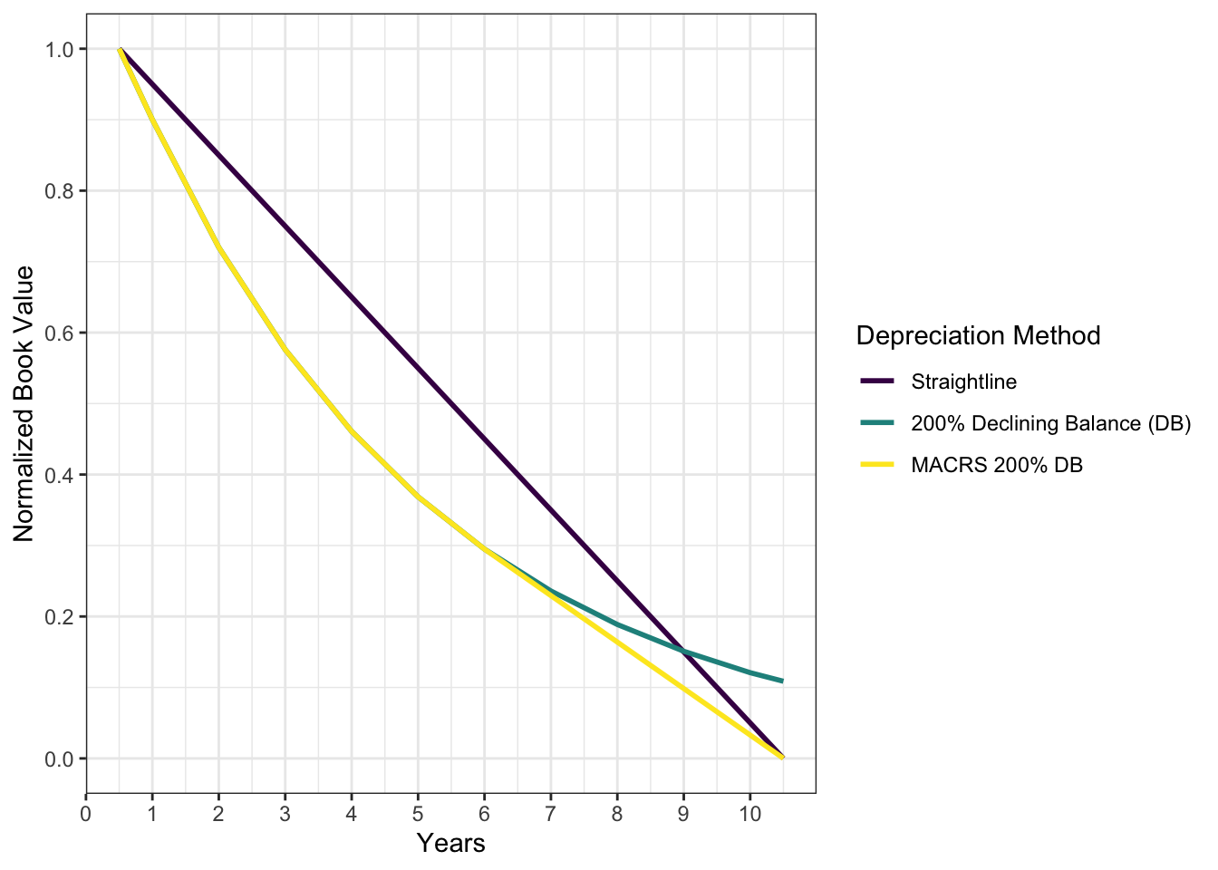
Figure 4.6 compares the normalized book value, \(BV_t/C\), for the straight-line method, a true 200% declining balance method and the MACRS 200% declining balance method over a 10-year return period. Using a true declining balance method the book value will never reach zero. Thus, the MACRS 200% declining balance method switches to a straight-line method when the straight-line results in a larger depreciation than the declining balance method. In a 10-year recovery with a 200% declining balance, this occurs at age 6 as shown in Figure 4.6.
The IRS (2024b) simplifies the depreciation calculations by providing tables of MACRS depreciation rates, \(d_{t,p}\), by different methods, years \(t\), recovery periods \(p\), and for the season when the asset began service. In addition, MACRS requires the book value to depreciate decrease all the way to $0 at the end of the recovery period for both straight-line and declining balance methods.
Note there are 11 years of depreciation factors for a 10-year recovery period in Table 4.6. This is because a half-year convention is used, meaning that we assume the asset is placed into service half-way through the first year \((t=0.5\ years)\), and ends half-way through the eleventh year \((t=10.5\ years)\) as shown in Figure 4.6. The first and eleventh year depreciation factors are 50% smaller than if they were full years.
In this course we provide depreciation factors for the MACRS 200% declining balance method using the half-year convention in Table 4.6. All the homework and exam problems regarding MACRS will use this table. The IRS (2024b) dictates the recovery periods for different classes of assets.3 The recovery period will be given you in your homework and exam problems. In your career you will need to consult IRS (2024b) or a certified accountant.
MACRS
Technically, MACRS defines both the straight-line and various declining balance methods depending on rates of depreciation and the seasons when the asset enters service, but many sources — including FE and PE reference manuals — use MACRS to refer to one particular declining balance method only. As in, they define two methods, straight-line recovery and MACRS. Pay attention to the context of the problem!
An important concept related to depreciation is the book value of the asset, or how much an asset contribute’s to your company’s overall value in a particular year \(t\). This is defined as
\[ BV_t=C-\sum_{n=1}^t{D_n} \tag{4.28}\]
Where
- \(BV_t\): Book Value in year \(t\)
- \(C\): initial cost
- \(n\): number of years in recovery period
- \(D_n\): depreciation in year \(n\)
Note that the book value is different from the market value — what the asset would likely sell for. For example, a the market value of a warehouse could appreciate from the purchase price due to rising real-estate prices, but for tax purposes the book value could decrease from the initial value, allowing the owner to take tax deductions on the decline in value of the warehouse. (Blank and Tarquin 2023a).
Which depreciation method should I use for my project?
The declining balance method will allow you claim larger deductions from your investments sooner. You can then use the money you save in taxes to recoup the costs of your investment, help pay off your loans of your capital investment, or invest in other projects.
If you have many other tax deductions in the earlier years of the recovery period, you may elect for one of the other methods that gives you larger tax deductions in later years of the recovery period.
4.7 Project Assessment
Learning Outcomes
- Identify preferred project alternatives using net present value, internal rate of return, and benefit/cost analysis.
In the previous section on returns, we looked at project evaluation largely as a binary consideration: is the IRR greater than the MARR? Or, is the NPV positive?
It is rare to only have one course of action in an investment. More typically, there are multiple different strategies or alternatives that you need to weigh against each other. In this section, we will discuss how to comparatively evaluate projects with different timelines, discount rates, and other variables.
The workhorse of this analysis is still the NPV and the IRR. Another common tool in this analysis is the benefit-cost ratio or \(B/C\). This effectively another way of describing the return on investment. All of these methods have strengths and limitations. They also sometimes identify different preferred alternatives.
NPV vs B/C vs IRR
If the projects are mutually exclusive (e.g. there are different alternatives for the same project, and you only can pick one alternative), then you might select the project with the largest net present value. This gives you the largest benefit.
If the projects are independent from one another (e.g doing project A doesn’t stop you from doing project B) then a good approach is to rank the projects by the IRR or B/C. First do the project with the best rate of return, if you have sufficient remaining funds, then do the project with the next best rate of return, and so on.
Other methods to rank independent projects projects given budget constraints are discussed in (Blank and Tarquin 2023b).
4.7.1 Non-monetary benefits and costs
To this point, we have considered that all the project costs and revenues are monetary: a company invests in a project, or an individual buys a house. But with public built environment projects, the costs and benefits might not always be monetary. For example, the Federal Highway Administration (FHWA) lists the following as potential benefits and costs that might be included in an analysis of a highway project(FHWA 2020):
- Travel time (and the reliability of travel time)
- Crashes
- Fuel use
- Vehicle operating costs
- Emissions/air quality
- Agency efficiency
The typical practice in the US has been to try and estimate these costs or benefits as monetary values and include them in the analysis. Many of these benefits and costs are difficult to monetize. Economists have developed prices for some of these intangible costs — such as the value of increased safety — by developing statistical costs of life or injury. For traffic crashes, one source of these estimates is the Highway Safety Manual (Transportation Research Board. Task Force on Development of the Highway Safety Manual and Highway Safety Manual 2010). Estimates of the societal costs of various types of traffic crash are given in Table 4.7 (recreated from HSM Table 7-1). These values include the cost of ambulances, medical care, property damage, lost productivity, and other similar costs. They explicitly do not include wrongful death or dismemberment damages resulting from civil court findings.
| Collision Type | Costs [2021 Dollars] |
|---|---|
| Fatal | $6,293,973 |
| Disabling Injury | $339,120 |
| Evident Injury | $124,030 |
| Fatal / Injury Combined | $248,374 |
| Possible Injury | $70,493 |
| Property Damage Only | $11,618 |
Think
Is it ethical to put a price on a human life when evaluating infrastructure projects?
Imagine what would happen if we planned all projects to try to eliminate all risks to zero. Despite our best intentions, we can never completely reduce the risks of dying due to building failure, traffic crashes, or exposure to harmful pollutants. Even if we did, we would not accept the costs of such actions. e.g. if everyone traveled at a max speed of 20 mph, we would likely save lives from traffic accidents, but the cost of the extra travel time would be too high.
Federal agencies such as the Federal Highway Administration (FHWA), and the US Environmental Protection Agency (US EPA) use the value of the statistical life (VSL) in benefit cost analyses of projects, programs, and rule makings. By using the VSL, we can monetize the benefits of increased safety or decreased exposure to pollution, to then choose an acceptable amount of risk by balancing both cost and safety.
The US EPA describes VSL as (EPA 2014)
The EPA does not place a dollar value on individual lives. Rather, when conducting a benefit-cost analysis of new environmental policies, the Agency uses estimates of how much people are willing to pay for small reductions in their risks of dying from adverse health conditions that may be caused by environmental pollution.
4.7.2 Risk Analysis
To quantify the potential benefits of avoided events, we need to better understand the risk inherent in those events. Risk is the probability that an event will occur, multiplied by the cost or impact of the event if it does occur. So in a population where events occur to an individual, the total risk is \[ \mathrm{Risk} = \mathrm{Population}\times P(\mathrm{event})\times\mathrm{cost\ of\ event} \tag{4.29}\] The units of risk are the same as the units of the cost or impact of the event. The benefit resulting from an improvement to the baseline condition is then calculated as the difference in risk between the two conditions.
Costs of avoided crashes
An intersection in Provo has an average traffic rate of 60,000 vehicles per day, and a fatal crash rate of 0.31 fatal crashes per million vehicles. A new design for the intersection would reduce the fatal crash rate to 0.28 fatal crashes per million entering vehicles and would cost $3 million to build.
In one year, what is the benefit of the new design in terms of reduced fatal crashes?
The value of the risk of the old system is given by looking at the economic costs of a fatal crash in Table 4.7 and using Equation 4.29, understanding that we have daily traffic but want an annual risk evaluation \[\begin{align*} \mathrm{Risk} &= \mathrm{Population}\times P(\mathrm{event})\times\mathrm{cost\ of\ event} \\ \mathrm{Risk}_{old} &= \left(\frac{60,000 \frac{\mathrm{veh}}{\mathrm{day}} * 365\mathrm{veh}/\mathrm{yr}}{1000000 }\right) \times 0.31 \frac{\mathrm{crashes}}{\mathrm{M veh}} \times 6,293,973 \frac{\mathrm{\$}}{\mathrm{crash}} \\ &= 42,729,783\\ \mathrm{Risk}_{new} &= \left(\frac{60,000 \frac{\mathrm{veh}}{\mathrm{day}} * 365\mathrm{veh}/\mathrm{yr}}{1000000 }\right) \times 0.29 \frac{\mathrm{crashes}}{\mathrm{M veh}} \times 6,293,973 \frac{\mathrm{\$}}{\mathrm{crash}} \\ &= 4e+07 \end{align*}\]
The benefits are the difference in risk, \[\begin{align*} B &= R_{old} - R_{new} \\ &= 42,729,783 - 4e+07 \\ &= 2,756,760 \\ \end{align*}\]
So, the annual benefit from this reduction in risk is $2,756,760. This is less than the cost of the project, but the benefits come every year for a one-time cost. So the project is probably worthwhile, but this wasn’t asked for in the problem.
Unknown costs
In all of the examples we have covered, the benefits and costs of the projects were taken as given. In the real-world, almost all of the revenues and costs can only be estimated. You should consider how confident you are in those estimates when conducting a financial or benefit cost analysis of a project.
4.7.3 Evaluation Matrices
While benefit cost analyses are useful, decision makers often consider additional factors regarding large infrastructure projects. Large public projects have benefits and costs that occur on a wide spectrum of different dimensions. It can be difficult or impossible to monetize all benefits and costs. Also, in a simple cost benefit analysis, we don’t consider social justice, or the equal sharing of costs and benefits (e.g. Who is benefiting the most from this project?, Who is most adversely impacted by this project?). We can use the triple-bottom line discussed in Chapter1 as a guide in making decisions, but within each of these dimensions can be multiple different variables that require consideration. A common method to put these variables into one decision making framework is by using an alternatives evaluation matrix.4 To create this matrix:
- Decide which elements of a project, in terms of benefits and costs or other outcomes need to be considered. This may involve public input.
- Develop a scoring system \(b\) for each element. This is often a score of 1 to 5 or a grade of A to F or some other categorical measure.
- Develop weights \(w\) for each element, again with public input.
- Calculate the weighted score of each alternative as \(S_a= \sum_e w_e*b_{ea}\) where \(S\) is the total weighted score for the alternative, \(w_e\) is the weight of each element \(e\), and \(b\) is the score of within that element for each alternative.
Figure 4.7 shows a project evaluation matrix from the Utah Transit Authority’s Point of the Mountain alternatives analysis. UTA has developed five different alternatives to provide high-frequency transit to Lehi and the site currently occupied by the Utah State Prison, using different combinations of light rail extensions and new BRT service. These five alternatives are each evaluated on a five-point scale applied to 19 different measures grouped into five general categories:
- Transit System Performance
- Access and Mobility
- Land Use
- Cost and Constructability
- Natural and Built Environment
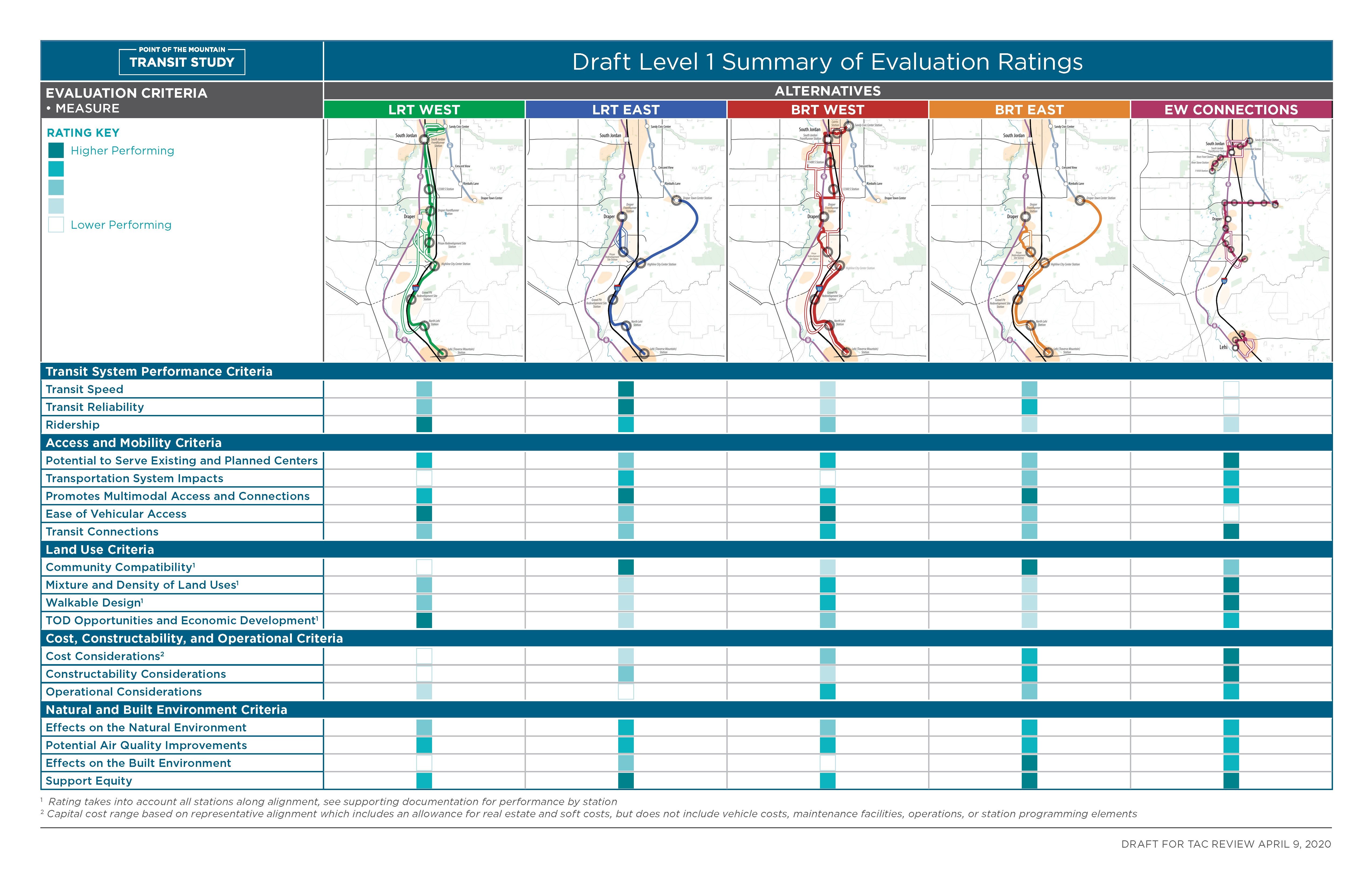
You can see in the figure how each alternative generally performs. The EW Connections alternative scores the best in terms of cost, but it performs poorly in terms of transit speed and reliability. The LRT East and BRT East alternatives have similar profiles, but the BRT option trades a bit of speed and reliability for a lower cost.
When conducted in this way, a number of different factors besides pure cost and benefit are allowed to contribute to the overall project evaluation. There is also a risk, however, that this method can become purely subjective if care is not taken to avoid pre-determining the outcome.
UVX
When the UVX system was constructed, there was a discussion about whether to access BYU from the west (on Canyon Road) or the east (on 900 East). Building it on Canyon Road was going to be cheaper and have a shorter overall travel time, but it would not attract as many riders.
| Criteria | Weight | Canyon Road | 900 East |
|---|---|---|---|
| Ridership | 0.3 | 1 | 3 |
| Cost | 0.2 | 2 | 1 |
| Travel time | 0.2 | 2 | 1 |
Identify the preferred alternative with the given weighting scheme.
To do this, simply multiply the value of each criterion in each alternative by the given weight, and sum by the alternative.
\[\begin{align*} S_a &= \sum_e w_e*b_{ea} \\ S_\mathrm{Canyon} &= 0.3 * 1 + 0.2 * 2 + 0.2 * 2 \\ &= 1.1\\ S_\mathrm{900E} &= 0.3 * 3 + 0.2 * 1 + 0.2 * 1 \\ &= 1.3 \end{align*}\]
Unit Summary
The time value of money means that $100 now is worth more than $100 in the future because of risk, inflation, and opportunity cost. This makes interest a powerful tool in funding projects with things like mortgages, bonds, sinking funds, and toll-based financing. Cash flow diagrams provide an easy way to organize the cash flows of projects over long periods of time. Using equivalence equations for present value, future value, and annuities allows us to calculate the net present value (NPV) from a cash flow diagram, which determines if a project will be profitable. We must pick an appropriate discount rate in order to correctly calculate the present value of future cash flows and to meet our minimum acceptable rate of return (MARR). We can also calculate the internal rate of return for complex cash flows from infrastructure projects.
Ultimately, though, decisions cannot be based on finances alone. They must also incorporate costs and benefits that do not have monetary values, either by determining a value for them or by using a suitable weighting system for different categories. Sustainable infrastructure can only be achieved if all of these factors are considered.
- annuity (A): a series of equal payments made over time
- benefit: A monetary or non-monetary advantage provided by a project or alternative
- bond: a financial tool in which an investor loans a sum of money to an organization, and the borrower pays annual interest on the loan until the end date of the bond, at which point they pay back the face value
- book value: the initial cost of an asset minus total depreciation
- cash flow diagram: a graphical display of cash inflows and outflows over time
- compounding frequency: the frequency with which the interest on a loan is re-applied to the principal
- depreciation: the value of an asset lost over time due to use, found using methods like straight-line or MACRS
- discount rate: an interest rate used to determine the present value of a future cash flow
- factor tables: tool for converting cash flows (PV,FV,A,G) into equivalent time values of money
- future value (F): the equivalent future worth of a sum of money or series of payments
- gradient (G): a series of equally increasing payments made over time
- inflation: the increase in price for goods and services over time
- interest: money paid by a borrower to a lender in exchange for the use of their money
- internal rate of return (IRR): the discount rate that makes the NPV of a project equal to zero
- minimum acceptable rate of return (MARR): the lowest rate of return that a project must earn in order to be worthwhile to an investor
- modified asset cost recovery system (MACRS): a set of methods for calculating depreciation values for assets
- mortgage: a loan to purchase property using that property as collateral, repaid in regular periodic amounts
- net present value (NPV): the equivalent present value of all future cash flows
- opportunity cost: the potential benefits that are lost when one option is chosen over another
- present value (P): the present worth of a sum of money or series of payments
- project assessment: comparing projects using methods such as NPV, ROI, B/C, and incremental B/C
- project evaluation matrix: a tool to compare several alternatives across an array of quantitative and qualitative criteria
- refinancing: taking out a second loan at a lower interest rate to pay off an original mortgage
- return on investment (ROI): the ratio of the equivalent annual earnings to the total investment
- risk: the chance that an investment will be less profitable than expected, including the possibility of losing some or all of the original money
- sinking funds: a fund where smaller amounts of money are put aside regularly to pay for some larger expense in the future
- time value of money: the concept that money now is worth more than the same amount of money later because of risk, inflation, and opportunity cost
Homework
Problem Set: Returns and ROI
HW 4.1: Investments and Returns
A corporation wants to build a renewable energy project with an expected capital investment of $750,000. During the life of the project, it is expected to generate $2 Million in revenue and cost $500,000 to operate. At the end of the project you expect to sell all remaining assets for $300,000. What are the returns and ROI for this project?
HW 4.2: Excavation Expansion
You own an excavation company. You are considering buying an additional excavator for $125,000 and hiring someone to operate it for one year. You will keep the excavator at the end of the year. With the excavator, you estimate your additional annual revenue and expenses to be:
| Revenue | Fuel | Maintenance | Insurance | Operator Wages |
|---|---|---|---|---|
| $120,000 | $10,000 | $10,000 | $15,000 | $50,000 |
What are the returns and ROI for buying the excavator?
HW 4.3: Excavation with a Loan
Now assume that you take out a loan to pay for the excavator. You have a 20% down payment and will pay $6,000 in interest. You don’t need to pay back the loan this year. All of the other expenses remain the same. What are the returns and ROI for buying the excavator with a loan?
HW 4.4: Excavation expansion: yes or no?
If you were in charge of this excavation company, should you expand by acquiring an additional excavator? Should you use debt and a bank loan to help make this expansion? What would be the risks of taking on debt? Write a short response below.
Problem Set: Taxes and Depreciation
HW 4.5: Book values
A company purchases a bulldozer for $200,000 and expects a salvage value of $30,000 at the end of the 7-year recovery period. Using both the straight-line and declining balance depreciation methods, calculate the depreciation and book value of the asset at the end of each year of the recovery period. Which method will have a lower tax burden in year 6, all else equal?
HW 4.6: Excavator Depreciation
Reconsider the excavator problem in HW 4 (where you took out the loan), but include the depreciation of your excavator and the taxes you need to pay to operate. Assume that the excavator has a 10-year lifetime with a salvage value of $10,000, and use straight-line depreciation. Use a 33% effective tax rate.
- What is the annual depreciation value?
- Re-calculate the annual returns and the simple payback period.
- Re-calculate the 1-year ROI considering the excavator depreciation.
HW 4.7: A fleet of excavators
Your company purchased an excavator in 2019, 2021, and 2022; each excavator cost $125,000. What is the total book value of all of your excavators in 2025 by the declining balance method? Construction equipment has a five-year recovery period.
Problem Set: Time Value of Money
HW 4.8: Time value F from P
A $5,000 investment earns 6% per year. What will be the value of this investment in 15 years if:
- The investment is compounded annually?
- The investment is compounded monthly?
HW 4.9: Time value P from F
When you were born, your grandparents purchased shares in a mutual fund paying 8% interest per year compounded annually, hoping that this investment would pay for your college tuition (lucky!). Assuming you are at BYU for eight semesters beginning when you are 19, how much should they have invested?
Assumptions
This problem requires you to make assumptions. There is not a single correct answer as different assumptions can be valid. Document your assumptions, and show your work.
HW 4.10: Comparing F
Sarah and Brian both invest in a retirement fund. Sarah invests $15,000 at age 30, while Brian invests $40,000 at age 50. Both accounts earn 8% interest per year, compounded annually.
- How much each will they each have at age 65?
- How much would Brian need to invest at age 50 to have the same amount as Sarah by age 65?
HW 4.11: Simple Uncle Shark
You borrow $20,000 from your uncle to help pay for four years of college (because your grandparents didn’t buy you a mutual fund…). You agree to a simple interest loan with an annual interest rate of 6% on the remaining principal owed at the end of each year. Each summer in college (before the end of the year) you work in his company and earn $4,000 which you use to pay down the loan principal. You then pay the entire loan off with your first out-of college paycheck at the beginning of year 5.
- How much total interest do you pay your uncle over the course of the loan?
- What is the payoff amount?
Include a table like the one below tracking your loan (you might find it helpful to have other columns as well).
| Year | Principal | Interest | Loan Balance (End of Year) |
|---|---|---|---|
| 1 | |||
| 2 | |||
| 3 | |||
| 4 |
HW 4.12: Compound Uncle Shark
Repeat the previous problem, but the loan is compounded annually. That is, the interest is calculated on the entire remaining balance rather than just the principal amount.
Problem Set: Annuities and Gradients
Tip
I recommend solving the problems in this problem set primarily with the factor tables in Appendix A, so you can get used to using them.
HW 4.13: Car Maintenance
Frank’s parents give him an old car that will last for 10 more years as long as he keeps repairing it. The car needs $500 worth of repairs the first year, and the maintenance costs will increase by $50 each year afterwards. How much money does Frank need to invest now at an 7% interest rate to pay for the next 10 years of maintenance on the car? Draw a cash flow diagram as part of your solution.
HW 4.14: Stock Market
You decide to invest in the US stock market, which has a historic return of 10% per year.
- How much would you need to invest each year to have $1,000,000 by age 65 if you started saving at age 25?
- How much would you need to invest each year to have $1,000,000 if you started at age 45?
HW 4.15: Depreciation in the present
You buy an excavator for $125,000 which has a 5-year recovery period and you expect to salvage the excavator for $25,000. What is the present value of all of the depreciation expenses if you use a straight line depreciation and assume a 6% discount rate? Include a cash flow diagram in your answer.
HW 4.16: Home Loan
You are buying a home for $430,000. Your 30-year mortgage has a 6.28% annual interest rate (compounded monthly) and requires a 20% down payment to secure.
- What is the monthly payment? Recall that \(i/k\) is the periodic interest rate.
- What is the total amount paid?
- For each month, calculate the amount of the payment that goes to interest and the amount that goes to principal. Create a plot showing these amounts over the entire course of the loan.
Help
Each month, your monthly payment includes part interest and part payment on your principal. If you pay all the interest that accrues each month, then any amount left over from your monthly payment will apply to the principal.
Set up a spreadsheet or computer program that calculates the amount paid to interest and to principal in each month of the 30-year mortgage. You should include example calculations and the top few rows of the table in your homework submission, but do not need to include the entire 360-line spreadsheet.
Also: if you have done this correctly, you will pay off the loan with your last payment.
HW 4.17: Home Loan Payoff
Consider the same information as the previous problem. What happens if you are able to pay an additional $200 each month?
- After how many years do you pay off the mortgage?
- How much total money do you pay?
- How much money do you save compared to the previous problem?
It is not necessary to include the graph again.
Problem Set: Equivalence
HW 4.18: Water lines
You are considering signing a contract to install water lines in a development project with a 5-year construction timeline. You expect your annual costs to be $400,000/year. The developer provides two options for your company’s payment.
- Option 1: The developer pays you $1,000,000 now (year 0), and $2,000,000 at the end of the project in 5 years.
- Option 2: The developer pays you $4,000,000 at the end of the project (in 5 years).
- Draw/graph a cash flow diagram of both options.
- Assume your company uses an annual discount rate of 12%. Calculate the present value for each of the payment options.
- Which is the preferred option using the net present value (NPV)?
- What other financial considerations are there that are not expressed in the NPV?
HW 4.19: Construction Company Present Value
You are a project manager for a construction company, and you are evaluating the potential investment in a new piece of heavy machinery. The initial cost of the machinery is $150,000. You expect this machinery to generate additional annual revenues of $45,000 for the next 5 years. At the end of the 5 years, the machinery will have a salvage value of $10,000. The company’s expected rate of return for their investments is 8%.
Calculate the Present Value of Future Revenues: Using the company’s expected rate of return of 8%, calculate the present value (P) of the additional annual revenues generated by the machinery over the next 5 years.
Calculate the Present Value of the Salvage Value: Calculate the present value (PV) of the salvage value of the machinery at the end of 5 years using the company’s required rate of return of 8%.
Calculate the Present Value of the Revenue and the Salvage Value: Combine the present value of the future revenues and the present value of the salvage value to determine the total present value (PV) of the revenues.
Determine the Net Present Value (NPV): Calculate the net present value (NPV) of the investment by subtracting the investment cost of the machinery from the present value of the revenue and salvage value calculated in question 3.
Evaluate the Investment Decision: Based on the NPV calculated in question 4, determine whether the company should proceed with the investment in the new machinery. Explain your reasoning.
HW 4.20: Air Conditioner
Alissa wants to install a new $9,000 air conditioning system. Because it is more energy efficient, the system would save $1,400 per year in electricity costs. Assume the air conditioner is installed in year 0, and savings begin with year 1.
- Without accounting for the time-value of money, what is the payback period?
- Assuming a discount rate of 7%, how long will it take for the air conditioning system to pay for itself? Assume the savings compound annually. Hint: Find the number of years where the net present value is 0. This problem can be solved in multiple ways: algebraically manipulating the formula to solve for \(n\), using goal seek to change \(n\), or plotting \(n\) vs. \(P\) in a table.
- Draw a cash flow diagram for each of the above parts. Make sure to label your axis and which diagram comes from which part.
HW 4.21: Bonds
Ben can buy a bond with a face value of $1,000 paying at 6% interest for five more years.
- Draw or graph a cash flow diagram for the bond.
- What is the present value of this bond if Ben’s personal discount rate is 5%?
- What is the present value at a 7% discount rate?
Note: to solve this problem, first draw the cash flow diagram for the bond. Then, determine the present value of the bonds using the different discount rates.
Problem Set: Internal Rate of Return
HW 4.22: Pavilion to rent
In 2019, you built a pavilion to rent for special events $15,000 and started operations in 2020. Each year you operate, you incur $100 in expenses. In 2020, you made no money because of the pandemic. But in 2021 you earned $1,000, and grew your business by an $1000 each year after (e.g. $2000 in 2022, $3000 in 2023, etc.). At the end of 2024, you sold the pavilion for $15,796.68.
- Draw a cash flow diagram of this project.
- Calculate the NPV of this investment given discount rates of 10%, 12%, and 18%.
- What is the IRR of this investment?
HW 4.23: Dock
You are considering building a new dock at a port. There are two options for the dock. Dock A is smaller, will cost $70 Million dollars, and will generate returns of $24 million dollars/year for the next 10 years. Dock B is larger. It will cost $170 Million dollars and generate $41 million dollars per year for the next 10 years.
- The port authority uses a discount rate of 8% to evaluate capital investments. What is the net present value of both options using the 8% discount rate?
- What is the internal rate of return for both options?
- Which dock would you recommend building? Why?
HW 4.24: Varying Incomes
In 2010, you made a $45,000 investment in new construction equipment, which you expected to generate revenue of $10,000 per year for the next ten years (2011 through 2020), on $3,000 of annual expenses. In reality, the revenue was the values in the actual column of the table below:
| year | expenses | expected | actual |
|---|---|---|---|
| 2011 | 3000 | 10000 | 7000 |
| 2012 | 3000 | 10000 | 10000 |
| 2013 | 3000 | 10000 | 13000 |
| 2014 | 3000 | 10000 | 18000 |
| 2015 | 3000 | 10000 | 11000 |
| 2016 | 3000 | 10000 | 2000 |
| 2017 | 3000 | 10000 | 8000 |
| 2018 | 3000 | 10000 | 12000 |
| 2019 | 3000 | 10000 | 7000 |
| 2020 | 3000 | 10000 | 14000 |
- Calculate the IRR for the expected project as well as what actually happened. Did things go better or worse than what you expected?
- Comment on what might happen in 2016 if this project was financed through a bank.
HW 4.25: The Big Kahuna
Difficult problem
This problem ties together almost everything you have learned in this unit. When you understand how to solve this problem, then you should be well-prepared for the test and to solve related problems in your career.
Advice to solve: clearly read the problem, and take each element in steps. Set up a spreadsheet to track each year’s returns, taxable income, and any values used to calculate those elements. As always, include example calculations in your homework response, alongside a replication of your spreadsheet.
Your company is looking to build a new incinerator that will generate electricity by burning household waste and thereby diverting trash from landfills. Someone in your office recommended calling this incinerator “The Big Kahuna” and no one else had any better ideas.
Each year you operate, you will generate electricity worth $1.5 million, and incur expenses of $400,000. Your incinerator will go online halfway through 2026, and will stop operations at the end of 2035 (i.e., 2026 will only have half the revenue and half the expenses but 2035 will have a full year).
The incinerator costs $3 million dollars, and you will finance its purchase with a bank loan offered at 6.5% annual interest compounded annually and 20% down, paid back over the next ten years (down payment in 2025, payments starting in 2026).
Incinerators like this one have a seven-year recovery period using the MACRS declining balance method. You also expect to salvage the equipment for 500,000 at the end of 2035. You pay a corporate tax rate of 28% on your taxable income, and your company has a MARR of 12%.
- Calculate the NPV of this project using a 12% discount rate.
- Calculate the IRR of this project.
Range of answers
If you have done this problem correctly, you should get an NPV in the neighborhood of $2.5 Million with an IRR between 50% and 100%.
HW 4.26: Self-financing the Big Kahuna
When you are about to finance the loan, one of the members of your board calls you up and says he would rather the company self-finance the incinerator purchase, to keep the company out of debt. Is this a good idea?
Tip
The best way to solve this problem is to simply copy your spreadsheet from the previous problem, and change it so that the entire cost of the incinerator comes up front, and remove the finance payments. Calculate the NPV and IRR, and use that information to tell your board member what you think the company should do.
Problem Set: Project Assessment
HW 4.27: Arizona Traffic Projects
You are evaluating the profitability of different traffic projects for the Arizona Department of Transportation (AzDOT). You assume that these projects will last a long time, and for simplicity you assume that the benefits can be projected for perpetuity (forever). The construction costs, and the annual returns from each project are listed in the table below. Assume that construction occurs at age 0 of the project, and the returns occur starting in year 1 for perpetuity.
| Project | Construction Cost | Annual Returns [M$] | Present Value (Returns) | Net Benefits | B/C | IRR |
|---|---|---|---|---|---|---|
| A | 20 | 1.8 | ||||
| B | 82 | 6.0 | ||||
| C | 120 | 10.0 | ||||
| D | 140 | 10.5 |
AzDOT uses a discount rate of 4% for all projects.
- Complete the table with these calculations. Show your work with an example calculation.
- Calculate the present value of the returns
- Calculate the net benefits
- Calculate the benefit/cost ratio
- Calculate the IRR (%)
Assume that projects A through D are for different independent traffic projects throughout Arizona. Your supervisor asks you to recommend which projects should be built this year given a budget of $140 Million. Which project(s) do you recommend? Which financial metric did you use to develop your recommendation? Hint: See the “Think” box in ?sec-npvirr.
Assume that projects A through D are different alternatives for the same traffic project. This means that you can only do one of the projects. Again you have a budget for this project of $140 Million. Your supervisor asks you to recommend one project. Which financial metric do you recommend to use? Why? What are your net benefits?
HW 4.28: Traffic Engineer in Provo City
You are a traffic engineer for Provo City. You recently conducted a safety analysis of pedestrian crossings. One of the pedestrian crossings was identified as University Avenue between the old Provo High school and the BYU Indoor training facility.
The pedestrian fatality rate was estimated to be 0.01 fatalities per 100,000 pedestrians. You estimate that 200,000 pedestrians will use the pedestrian crossing per year. Assume that Provo City uses a value of a statistical life of $11,000,000.
You have developed two different proposals for the city. Option 1 is an elevated walkway, and Option 2 is an improved crosswalk with flashing lights. You have conducted a safety analysis of both options. Option 1 is the safest option, but the most expensive. Option 2 improves the safety, but is much less expensive. The lifetime of both projects is assumed to be 30 years.
| Project | Fatality Probability per 100,000 Pedestrians | Construction Costs |
|---|---|---|
| baseline | 0.0100 | 0 |
| Option 1 | 0.0010 | 4,000,000 |
| Option 2 | 0.0075 | 600,000 |
- Calculate the annual cost of the risk of pedestrian fatalities in dollars, assuming 200,000 annual pedestrians, estimated pedestrian fatality rates, and the value of a statistical life. From the baseline scenario, and the two proposals. Use the definition of risk found in Equation 4.29
- Calculate the benefits for each of the two proposals as the reduced risk of pedestrian fatalities over the 30-year life-time of the pedestrian crossings. Calculate the benefits as the reduction in risk from the baseline scenario. Calculate the present value of benefits over the 30-year lifetime of the pedestrian crossings. Use a discount rate of 2%.5
- Calculate the net benefits (Benefits – Construction Costs) for the lifetime of the project. Which project has the higher net benefits?
- Calculate the benefit/cost ratio for the lifetime of the project. Which project has a higher benefit/cost ratio?
- From the financial perspective, are both options worth considering? Why?
- Which project would you recommend? Why?
Problem Set: Multi-criteria
You can also see this as an algebraic operation, \(F = P * F/P (i, n)\), where the factor you want \(F\) is isolated by dividing \(P/P\).↩︎
This isn’t how PhDs work in engineering, where your tuition is usually paid by your research grants.↩︎
For example, tractor units have a recovery period of 3 years. Vehicles have a recovery periods of 5 years. Office furniture, railroad tracks, and natural gas lines are 7 years, land improvements, electric transmission properties are 15 years. Water treatment and water distribution properties are 25-years. As you can see the recovery periods only seem somewhat related to the actual life-time of the assets.(IRS 2024b)↩︎
This is sometimes called a Kepner-Tregoe (KT) matrix after the authors who proposed it as a rational process for decision making (Kepner and Tregoe 1981).↩︎
When we conduct a lifecycle analysis, shouldn’t we calculate the future value of cost and benefits to account for inflation, and then discount it back to the present value? In other words, if a VSL is worth $11 million today, shouldn’t it be worth even more in the future? The White House’s guidance on conducting lifecycle analysis recommends using constant-dollar values for future costs, and use a discount rate that has the inflation effect removed, called the real discount rate. The nominal discount rate is an estimate of the time-value of money, including the impact of inflation. For regulatory analysis, the White House recommends estimating the nominal discount rate from US treasury returns (OMB 2023). The real discount rate is calculated by subtracting the impact of inflation rate from the nominal discount rate. For example, if the nominal discount rate is 4%, and inflation is 2%, then the real discount rate is approximately 2% (See ?eq-discount). The net present value will be the same if your future costs include an inflation rate of 2%, and you discount using the nominal rate of 4%, as a case where future costs are expressed in constant-dollars, and you discount back to the future using the 2% real discount rate.↩︎