Unit 2 Economics
You buy lots of things. From the shoes to your feet to the mask on your face, almost everything you can see or touch was purchased. If not by yourself, than by someone else. Some things you buy and then own. Other things you pay a fee to rent. Other things are services or experiences that you can buy.
You will also sell lots of things throughout your life. Obviously if you are in a trade that produces goods, you will sell those goods. There will also be occasions where you will sell something you are no longer using, be it a tennis racket at a yard sale, or a car you have replaced, or a home you no longer live in. But as an engineer the thing you will sell most frequently is your knowledge and skills through your labor. Someone will pay you for expertise and time that they do not have, and in exchange you will buy the things you and your family and your business need to keep going.
The sum total of all of these buying and selling transactions in a society is called the Economy, and economics is the branch of social science that studies these transactions.
Looking at the world from a purely economic perspective — the idea that anything in this world can be purchased with sufficient funds — is at once true and supremely corrupting / discouraging. Money is a necessary evil of our world, and it (almost) always has been. But understanding how the economy works is necessary to succeed in life and help yourself and those around you overcome the world. Some teachings on money from the Savior:
And I say unto you, Make to yourselves friends of the mammon of unrighteousness; that, when ye fail, they may receive you into everlasting habitations. — Luke 16:94
Lay not up for yourselves treasures upon earth, where moth and rust doth corrupt, and where thieves bbreak through and steal: But lay up for yourselves treasures in heaven, where neither moth nor rust doth corrupt, and where thieves do not break through nor steal: For where your treasure is, there will your heart be also. —Matthew 6:19-20
2.1 Supply and Demand
Let’s say people want to buy widgets. People will buy a certain number of them based on how much they cost. If the price is low, people will buy lots of widgets. If the price is high, people will not buy as many. This demand function \(P = D(Q)\) might look like this:
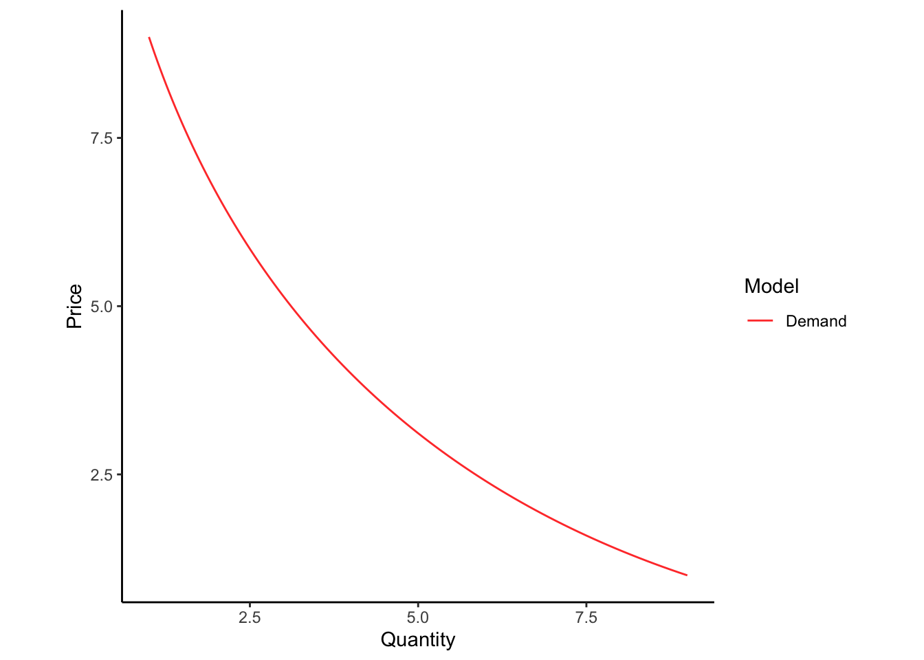
The slope of the demand line is related to a meaningful economic concept called the elasticity. Mathematically, elasticity is defined as the percent change in the quantity demanded resulting from a percent change in the price.
\[\begin{equation} \varepsilon = \frac{\%\Delta Q}{\% \Delta p} \tag{2.1} \end{equation}\]
When the price of gasoline was $2.45 per gallon, the average driver in Utah used 11.3 gallons per week. When the price increased to $2.55 per gallon, the average driver in Utah cut out a couple of unnecessary trips and used 11.2 gallons per week. What is the elasticity?
We just need to calculate the percent change in these values
\[\begin{align*} \varepsilon & = \frac{\%\Delta Q}{\% \Delta p}\\ &= \frac{(Q_1 - Q_0)/Q_0}{(P_1 - P_0)/P_0}\\ &= \frac{(Q_1 - Q_0)P_0}{(P_1 - P_0)Q_0}\\ &= \frac{(11.2- 11.3)2.45}{(2.55- 2.45)11.3}\\ &= -0.217 \end{align*}\]
Some goods are elastic, meaning that a small change in price results in a large change in demand, (\(\varepsilon < -1\)). Other goods are inelastic, meaning that demand will remain more or less fixed as the price goes up (\(-1 < \varepsilon < 0\)). Goods where the demand actually increases at the price goes up (\(\varepsilon > 0\)) exist, but are very unusual.
Are there goods that you will buy no matter what the price is? For lots of people, things like milk, gasoline, and diapers fit in this category.
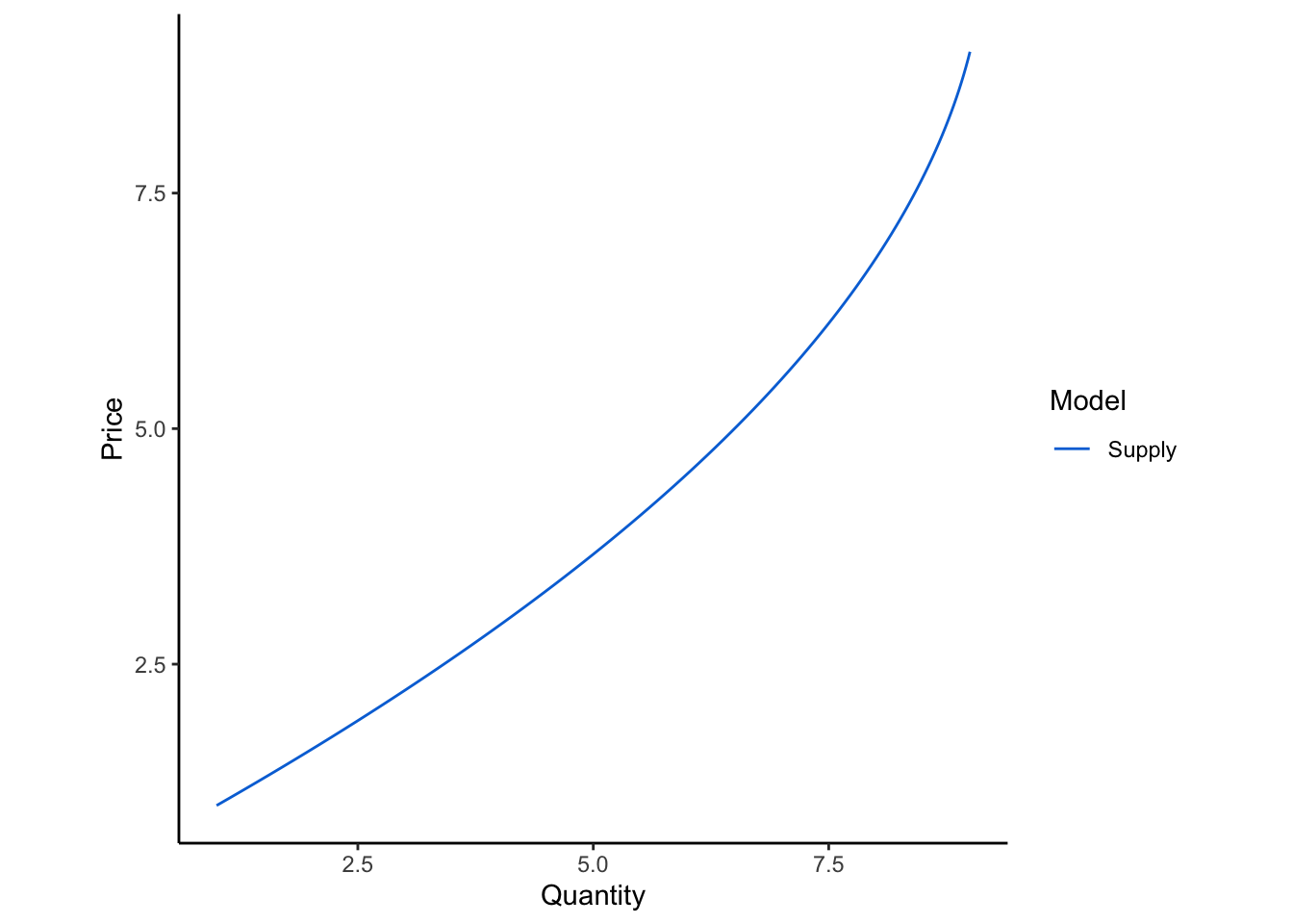
Somewhere else in the economy, there are people who make widgets. These people have exactly the opposite incentives as the people in the demand function. If the price of widgets is high, manufacturers will want to sell lots of them. If the price is low, then manufacturers will not make as many. This supply function \(P = S(Q)\) looks like this:
When we put both functions on the same plot, you can see that there is a particular price where the demand and supply curves intersect. If manufacturers set a higher price than this equilibrium point, they will make more widgets than people will buy. If manufacturers set a lower price point, they will run out of inventory and lose revenue. Note that this solution also sets the quantity of goods that should be manufactured or purchased.
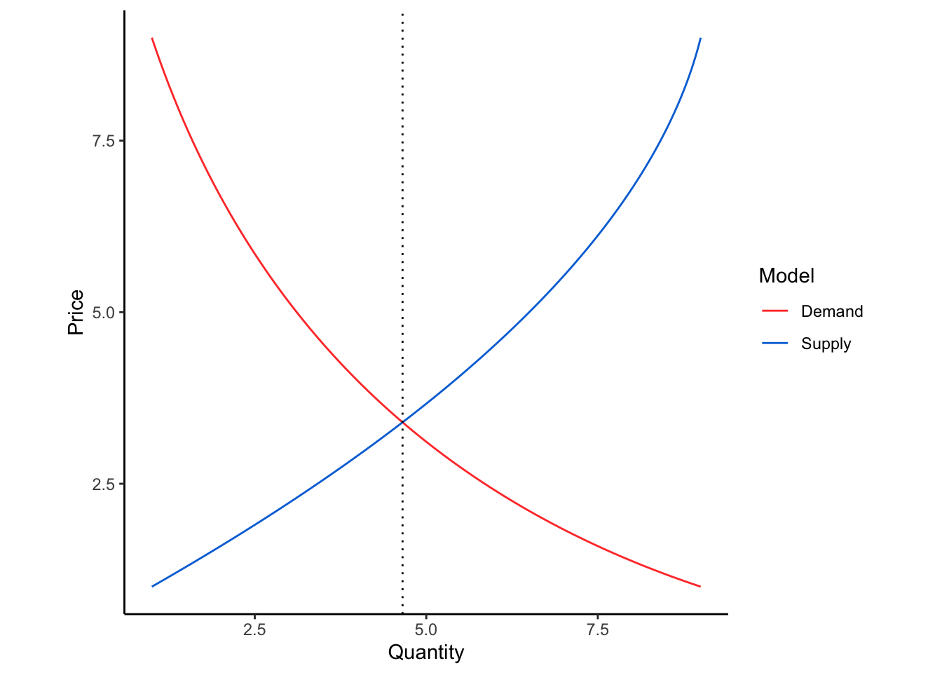
Finding the intersection of the supply and demand functions requires some simple algebra. You are looking for the solution \((Q, p)\) of the system of equations
\[\begin{equation} \begin{cases} p = S(Q) \\ p = D(Q) \end{cases} \tag{2.2} \end{equation}\]
This is most easily done by setting the difference of the functions equal to zero \(S(Q) - D(Q) = 0\) and then solving one of the other equations for \(p\).
The demand for a good can be described by the function \(p = 2/Q\). The supply of the good can be described by the function \(p = 0.5Q\). What is the equilibrium price and the quantity sold / purchased?
We need to find the solution to these two functions.
\[\begin{align*} \frac{2}{Q} &= 0.5Q\\ 2 &= 0.5 Q^2\\ Q &= \sqrt{4}\\ &= 2 \end{align*}\] And if \(Q = 2\), then \(p = 1\).
Supply and demand functions change over time. Sometimes the reason is obvious, and sometimes it is not. If the population grows, then there will be more people who want to buy widgets. This will push the demand for widgets upwards. If nothing else changes in the supply function, then the price will rise and more widgets will be produced / purchased.
If the population grows by 10%, a simplifying assumption would be that the entire demand curve also increases by 10%, \(p = 1.1 * D(Q)\).
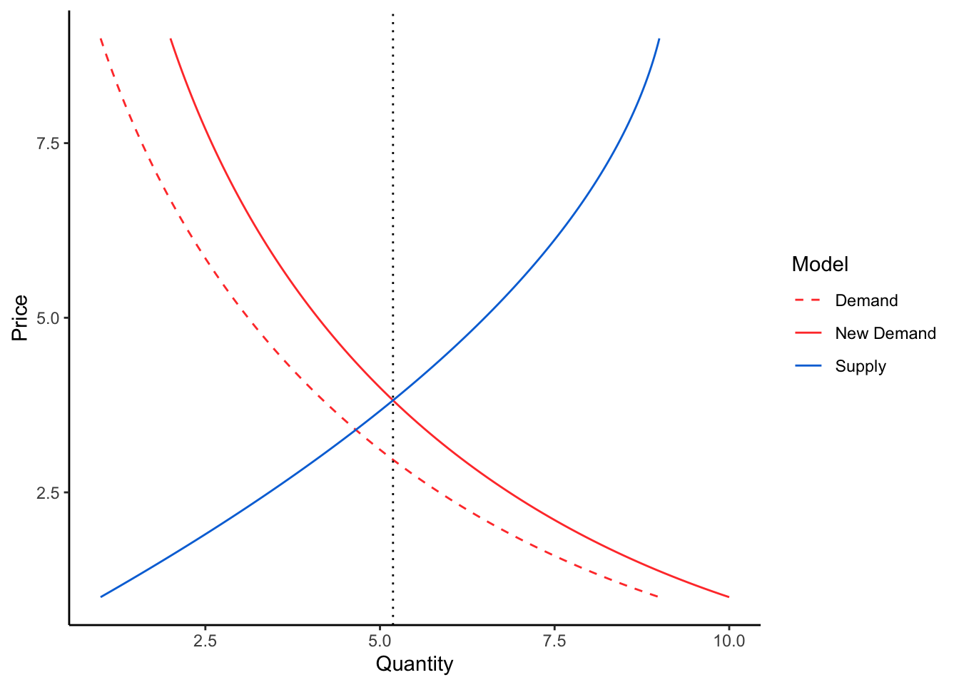
Sometimes the supply function will move up as well, meaning the system could reach the same equilibrium price for widgets as before. But often, the manufacturers have sufficient market power to increase supply while holding the price a little bit higher than before. This results in inflation, or the nominal price of goods creeping upwards. When wages increase to match price inflation, you have the tendency for currencies to lose purchasing power over time.
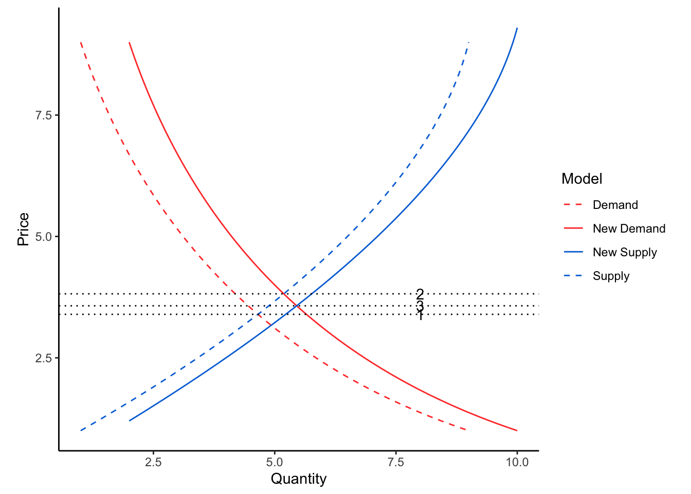
Inflation is often seen as a bad thing, because it means that a dollar you have now will not buy as much as in the future. But what happens when there is price deflation? Or what if inflation was exactly zero?
2.2 Utility
Think about the last time someone gave you a cash gift. Immediately, you started thinking about what you would want to purchase with that money. You realized that if you bought one thing, then you could not also buy another. This is the opportunity cost of the transaction. So how do you decide which thing to buy with your limited budget.
Utility is the value that an individual assigns to a particular choice. For example, if you purchase an orange, you have decided that the utility of consuming an orange is greater than the utility of consuming something else, or the utility of saving the money for a different purchase. In this analogy, the pleasure and nutrition you gain by eating the orange is the utility, while the price you pay for the orange is considered a disutility. If we believe that people are rational, then they will always choose the alternative with the highest utility.5
Let’s consider that we have two goods6 we want to purchase: \(x\) and \(y\). We get utility by purchasing these goods, and we get more utility by purchasing more of them. In the graphic below, any combination of \(x\) and \(y\) in the shaded area results in more utility than the point \(x^*, y^*\). Similarly any point below and to the left of that point results in less utility.
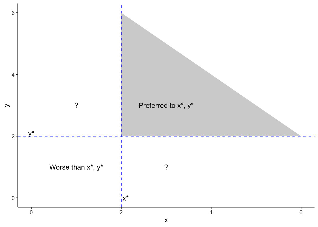
What is unclear, however, is how someone might view points in the areas marked by ?. This depends on how individuals might prefer a little bit more of \(y\) to a little bit more of \(x\). A mathematical equation that shows different combinations of \(x\) and \(y\) resulting in a single value of utility is called an indifference curve. For example, let’s view the indifference curves for three different values of utility if the utility function is \(U = xy\).
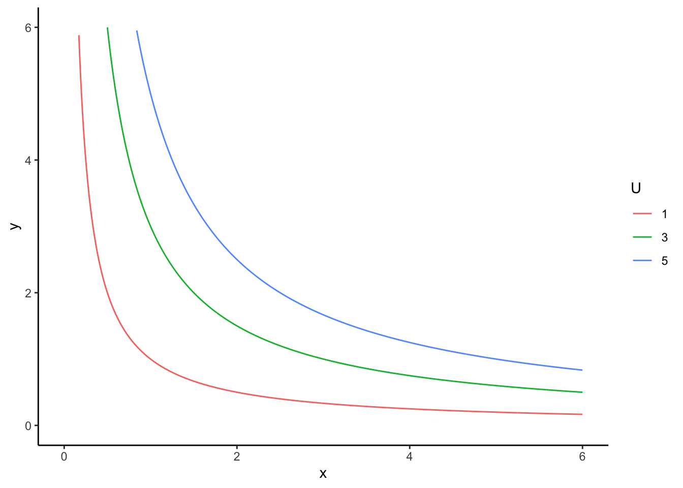
Any combination of \(x\) and \(y\) along a line of the same color gives exactly the same utility. And any point along the blue line has a higher utility than any point along the red line.
In this example, note that as you move away from the curve the slope \(dx/dy\) becomes more constant. What does this mean in terms of the utility gained by trading \(x\) for \(y\)?
We have a certain amount of income \(I\) that we will allocate to these two goods, and we can buy quantities of these goods in continuous amounts. Given a price for each good \(p_x, p_y\), the highest quantity \(Q_{max}\) we could buy for either good is
\[\begin{align*} Q_{max,x} &= I / p_x\\ Q_{max,y} &= I / p_y\\ \end{align*}\]
but only if we purchased none of the other good. Let’s visualize this graphically.
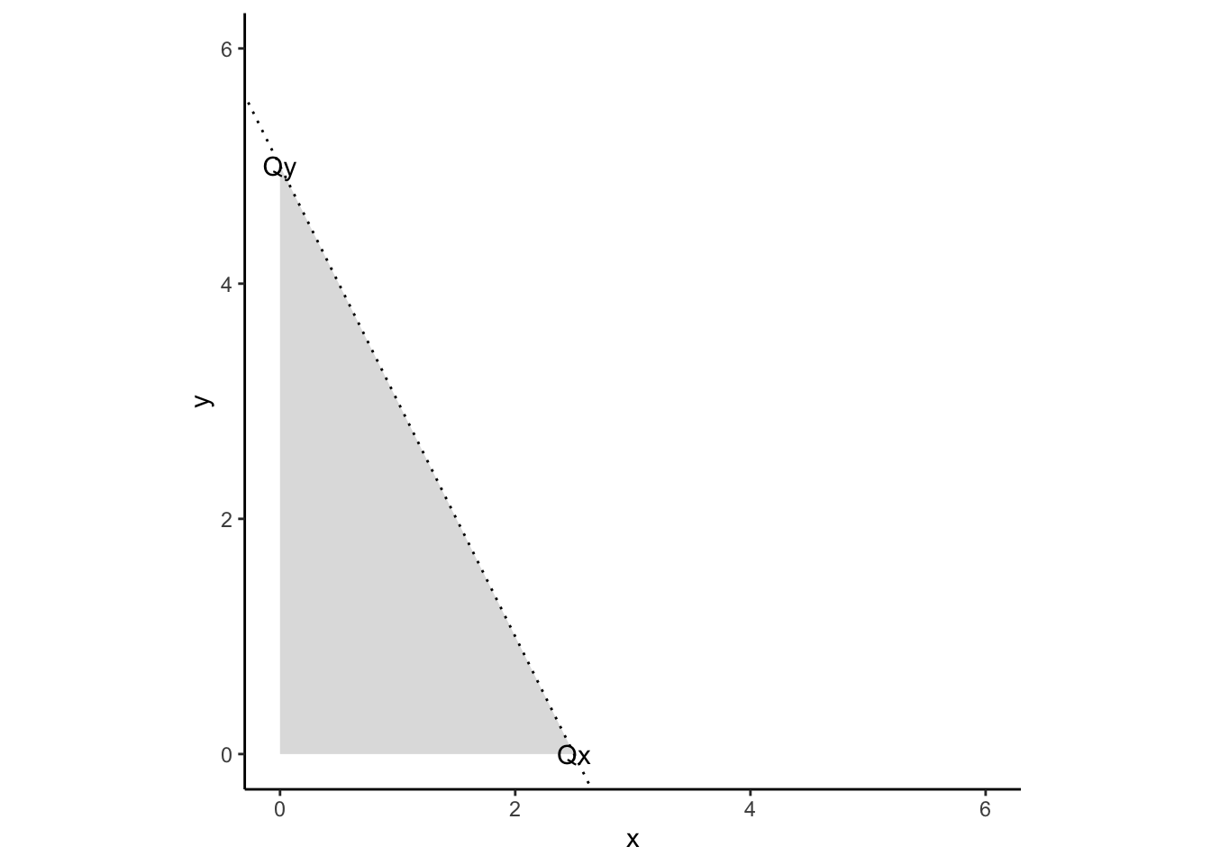
The dotted line represents the budget; there is no combination of \(x, y\) beyond this line that is permitted by the budget constraint \(I\). The points in the shaded region are allowed by the budget:
\[\begin{equation} p_x x + p_y y \leq I \tag{2.3} \end{equation}\]
Now, let’s plot the our indifference curves on top of our budget constraint. The point where the budget constraint intersects with the green indifference curve is the point that a rational actor will choose.
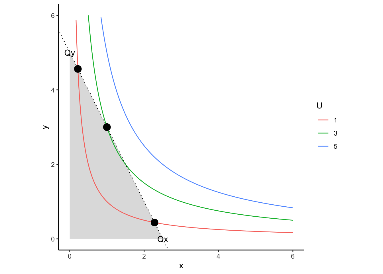
What will happen if the price of good \(x\) decreases?
This is a constrained optimization problem. There are several basic ways to solve these kinds of problems, depending on your skills and the difficulty of the problem.
- If you have had multi-variable calculus, you can find the analytical maximum utility point using the Lagrangian. Wow, look, a real application!
- You can use a numerical optimization routine contained in a software package like R, python, or Matlab.
- You can also use Excel’s Solver.
You have a budget of \(I = 5\), to split between two goods, \(x\) and \(y\). The prices of these goods are \(p_x = 2\) and \(p_y = 1\). The utility function for these goods is \(U = xy\), and you can buy these goods in continuous amounts. What is the combination of quantities that maximizes utility?
The maximum amount of either good we could purchase is either \(x = I / p_x = 2.5\) or \(y = I / p_y = 5\). But in either case, the Utility is zero because \(U = 2.5 * 0\). I’m going to present the solution in Excel using the solver.
If you would like to use R to find a solution to a constrained
optimization problem, the Rsolnp library works well.
library(Rsolnp)

# objective function: maximize utility on two goods
#  x: amount[1]
#  y: amount[2]
utility <- function(amounts){
  -1 * amounts[1] * amounts[2]
  # most functions actually perform *minimization*, so we will find the minimum
  # of a negative utility
}

# constraints: subject to budget constraint
budget <- function(amounts){
  2 * amounts[1] + amounts[2] # price of x is 2, price of y is 1
}

# find the solution of the problem
optimal <- solnp(
  c(0, 0), # starting values for search
  utility, # objective function
  eqfun = budget, eqB = 5 # constraint: the budget must be spent
)
##
## Iter: 1 fn: -3.3797 Pars: 1.47942 2.28447
## Iter: 2 fn: -3.1250 Pars: 1.25000 2.50000
## Iter: 3 fn: -3.1250 Pars: 1.25000 2.50000
## solnp--> Completed in 3 iterations2.3 Comparative Advantage and Trade
It is not conceivable that one person could learn everything there is to know in this life. And even if someone tried, little time would be left for anything else. Everyone has unique talents, interests, and skills that they have developed. By selling skills and knowledge that you have to people that don’t, you can earn a living. Money is a key component in this. A university professor cannot easily purchase groceries by volunteering to lecture the checkout clerks. Instead, university students pay tuition7 in exchange for a chance at a degree. The university then pays the professor a salary to teach and research, and the professor can then go to the grocery store and buy food for his or her family.
Of course, some people are better at doing some things than others. As much as a professor might rather be a professional tennis player or a sponsored fly fisherman, enough other people are more skilled at those endeavors to match all the demand that exists. The professor’s comparative advantage is to teach engineering and economics to university students, because the professor can do that better than the other people who want to be professors.
The theory of comparative advantage doesn’t mean that every job is done by the person who can do it best. A professional tennis player might be a better engineering professor than the person who is actually an engineering professor. But the tennis player is making more money as an athlete, and their comparative advantage lies there. The athlete’s comparative advantage is playing tennis, and professor’s is being a professor. This is simply another form of opportunity cost, as we discussed above.
Comparative advantage plays an important role in infrastructure, as it is the underlying process driving a great deal of the world’s transportation. Imagine a town with no transportation infrastructure: everything the town needs must be produced in the town. There will be lots of things that people in the town would want to buy, but there is no one with the time to produce it. But after engineers connect the town to the world economy by building ports, roads, railroads, airports, warehouses, and everything else, the comparative advantage changes. Suddenly goods that were expensive to produce in the town can be imported for a lower cost. This means that people can buy the cheaper goods, and the person who used to make those goods will find a new area in which he or she holds a comparative advantage.
How does automation in manufacturing change an economy in the context of comparative advantage?
Region \(A\) can make cloth cheaply, but cannot produce dairy products like milk and cheese because the terrain is unsuitable for dairy farming. The 320,000 residents currently use 24,000,000 pounds of clothes which they make at $1.33 per pound, and 32,000,000 pounds of dairy products which they buy for $2.5 per pound.
Region \(B\), on the other hand, has many high-quality dairy farms, but lacks the material necessary to produce clothing. The 400,000 residents currently buy 30,000,000 pounds of clothes for $2 per pound and produce the 40,000,000 pounds of dairy products they use for $1.5 per pound.
Currently, the two regions have no trade with each other. If a road were built between the regions, the cost of transporting dairy products would become $0.15 per pound, and $0.1 per pound of clothing. If the two regions began trading with one another, what would the economic benefits be for Regions \(A\) and \(B\)?
The answer is found by comparing the regions’ current costs with their potential costs if they trade. Region \(A\) can produce the clothing Region \(B\) needs for much cheaper, and Region \(B\) can provide the dairy products Region \(A\) needs for less than their current costs. The cost of dairy in region \(A\) before and after trade can be calculated as
\[\begin{align*} \text{Without trade:}& 32,000,000~lbs*\$2.5/lb=&\$80,000,000\\ \text{With trade:}& 32,000,000~lbs * \$(1.5+0.15)/lb=&\$52,800,000\\ \end{align*}\]
| Region | Without Trade | With Trade | Benefits |
|---|---|---|---|
| A Dairy | $ 80,000,000 | $ 52,800,000 | $ 27,200,000 |
| B Clothes | $ 60,000,000 | $ 43,000,000 | $ 17,000,000 |
This analysis shows that Region A would benefit $27,200,000 by trading with \(B\) for dairy products instead of producing them internally. Similarly, Region B would gain a $17,000,000 benefit. Further, the benefits that go to consumers in Region A would be in addition to the extra business for producers (because the money consumers used to spend in Region B would be used to buy goods from Region B). Even though Region A gains more than Region B in this situation, both would be winners for working out this arrangement. Further, if the road costs less than $44.2 million to build, it makes economic sense to build it. It would be important to make sure that the costs are borne equitably between Region A and B, so that the system can be socially sustainable.
This example is drawn from Fricker and Whitford (2019), and used with permission.
2.4 Public and Common Goods
A good in an economy is something that can be owned or consumed by people; these can be actual products, or they can be services. Goods can be classified based on two primary characteristics:
- Exclusivity: Can someone be effectively prevented from using a good if they did not pay for it?
- Rivalry: Does using a resource prevent others from using it? Or does using it diminish the experience of tohers.
These two characteristics form a matrix of four types of goods, shown in Figure 2.1. Private goods are rivalrous and exclusive. Most goods in the economy are like this. A grocery store requires that people pay for food before leaving with them (exclusive), and food that is consumed by one person is not consumed by other people (rivalrous). Goods that are exclusive but not rivalrous are sometimes called “club” goods: streaming services and cable internet are usually unaffected by the number of people watching them, but you have to have paid a login to get them.
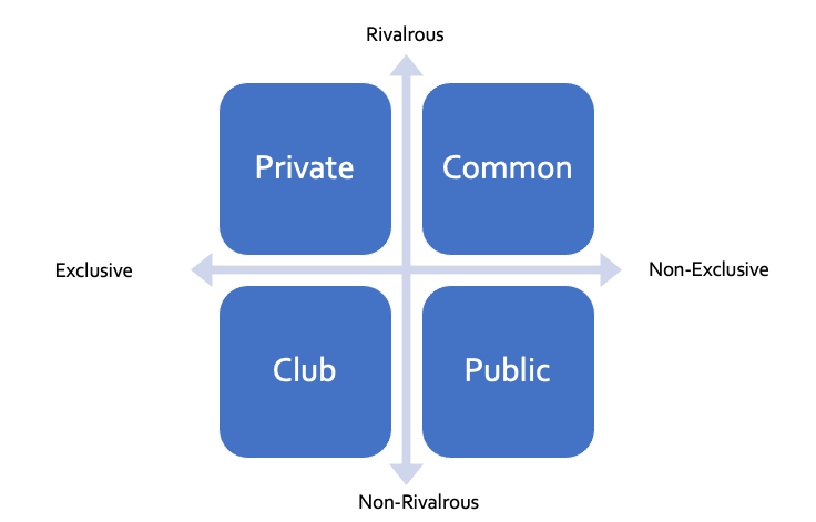
Figure 2.1: Types of goods by exclusivity and rivalry.
Public goods on the other hand are non-exclusive and non-rivalrous. A standard example of a public good is a light house. If you own a light house overlooking a harbor, there is no way for you to only allow ships that have paid a fee to see and use your light house (non-exclusive). If one ship is currently using your light house, other ships can use it at the same time (non-rivalrous). So if you own a light house, you probably need to find some other way to pay for your salary besides a subscription. In the United States, light houses are often operated by the Coast Guard as a public service.
In fact, much of the infrastructure in the United States is provided as a public good. Our lives are better and more prosperous because of this infrastructure, but it is sometimes hard to convince people to pay taxes to fund it.
Consider two roommates who share certain household supplies like toilet paper and cleaning chemicals. These will be considered a “public good” that benefits both roommates. Roommate 1 has the following utility equation:
\[U_1 = \sqrt{x_1 + x_2} * \sqrt{y_1}\]
Where \(x_1\) is the amount of shared supplies that Roommate 1 purchases, \(x_2\) is the amount that Roommate 2 purchases, and \(y_1\) is the amount of private goods that Roommate 1 purchases (foods, clothes, etc.). The budget for Roommate is given as
\[300 = 10x_1 + y_1\]
The combination of \(x_1, y_1\) that maximizes Roommate 1’s utility subject to this budget constraint turns out8 to be a system of the following equations:
\[y_1 = 10(x_1 + x_2)\]
\[x_1 = 15 - x_2/2\]
If Roommate 2 buys more shared supplies, then the amount that Roommate 1 wants to buy goes down. If \(x_2 = 20\), then \(x_1 = 5\), and then \(U_1 = \sqrt{25}\sqrt{250} = 79\). This is called the free rider problem.
But in reality, Roommate 2 is playing the same game, with an optimal \(x_2 = 15 - x_1 / 2\). Solving the entire system together and calculating the utility, we get \(U_1 = U_2 = \sqrt{10 + 10}\sqrt{200} = 63.2\)
BUT
What if the roommates instead pooled their resources to buy the supplies? The two utility equations remain exactly the same, but the budget constraint is now
\[600 = 10x + y\]
In this case, it can be shown that the maximum utility point is at \(y = 10x\). Putting this into the budget constraint gets us \(x = 30, y = 300\), and the utility for each roommate is now \(U_1 = U_2 = \sqrt{30}\sqrt{150} = 67.1\)
So both roommates will have a higher utility (and be better off!) if they share resources and coordinate their purchase of public goods rather than compete with each other and hope the other guy pays.
Public goods are often owned by the public through governments, but not always. AM and FM radio and broadcast TV are all non-rivalrous and non-excludable. But just because they are public goods does not mean they are free; you pay to listen to the radio or watch TV by spending a good portion of your time in advertisements.
2.4.1 Tragedy of the Commons
Common goods are like public goods in that they are non-excludable. But common goods are rivalrous: not everyone can use the resource at the same time. Common goods can quickly become a sustainability issue. Usually, economists tend to believe that people following their own self-interest helps to set fair prices and encourages innovation and diversity in the economy. But if private interests encourage someone to over-use a common resource, then the resource could become degraded or disappear. This phenomenon — that private short-term interests conflict with long-term social interests — is called the tragedy of the commons.
The video below shows how the tragedy of the commons might play out in a village fishing pond; if people catch fish more quickly than they can regenerate, the pond will eventually have no fish. The public interest is in keeping the fish pond operating, but the private interest of each person is to catch as many fish as they can.
Figure 2.2: Tragedy of the Commons
The Tragedy of the Commons can happen whenever private interests and public interests are in conflict. Examples or scenarios include the following:
- Fisheries in the North Atlantic depleted by overfishing
- Rain Forests destroyed for private agriculture
- Excessive lumber extraction from national forests
- Consuming irrigation water for high-water crops in California
Fixes for the Tragedy of the Commons usually require some kind of societal intervention. State fishing licenses limit the number of people who can fish, place catch limits on those who do, and provide resources for government enforcement and restocking efforts. Of course, knowing what interventions to install and how to shape them is a complicated problem.
Do we think of roads and streets as a private, common, or public good? Is this how they actually work? What are the consequences of this classification?
2.5 Externalities
Imagine you are riding your bicycle down a road when a large truck drives by “rolling coal”. As you inhale the noxious fumes, you suffer from this experience. And the truck drives on — perhaps oblivious to your coughing and perhaps not — without paying you anything for the costs his actions put on you.
It is common for the actions of one person to affect others. Sometimes these costs are captured within a market transaction, but other times they are not. Costs that are not captured within a transaction are called externalities because they are external to the transaction. When I put fuel in my gas tank and burn it, the market transaction is between me and the gas station / oil company. But everyone in the area breathes a little bit of my exhaust, and I’m not paying anyone to do that. Similarly, if I choose to stop buying gas and ride my bike, I still have to breathe the same polluted air as if I were driving.
So what can be done? In economic theory, the market sets the optimum cost of gasoline too low; the cost of pollution is not included in the transaction between the driver and the gas station. This means that there is some discrepancy between the market-established supply curve and a socially-optimal supply curve. If we implement a tax that moves the price of the from the the market price to the social optimum price, then the external costs can be captured and returned to the public.
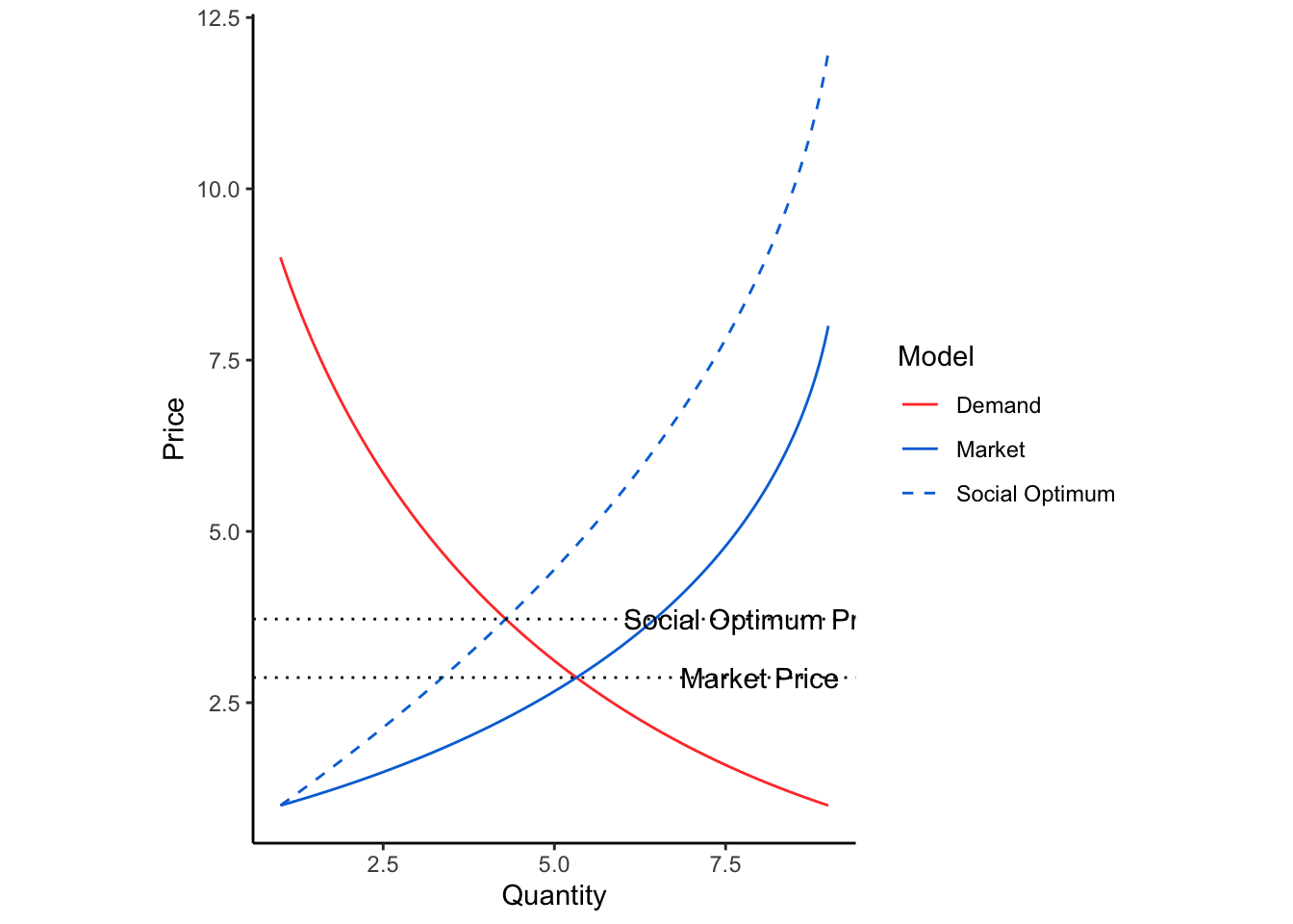
Demand for electricity is defined by the equation \(D(Q) = 4/Q\). The market-determined supply function is \(S(Q) = 1.2Q\), but the socially optimal supply function is \(S'(Q) = Q^2\). Find the equilibrium price and quantity consumed under market the conditions and under socially-optimal conditions, and the tax required to acheive this optimum.
The market equilibrium can be found by setting \(D(Q) = S(Q)\):
\[\begin{align*} 4/Q &= 1.2Q \\ Q^2 &= 3.33\\ Q &= 1.826\\ \end{align*}\] implying that the equilibrium market price is \(4/1.826 = 2.19\). The socially optimal equilibrium, however, is at \(D(Q) = S'(Q)\): \[\begin{align*} 4/Q &= Q^2 \\ Q^3 &= 4\\ Q &= 1.587\\ \end{align*}\] and the equilibrium social optimum price is \(4/1.587 = 2.52\). The tax therefore is \(2.52 - 2.19 = 0.33\)
Unit Summary
A good introductory resource on many of the topics in this unit is Khan Academy’s Microeconomics course.
- Economy The sum of all transactions in a society.
- Supply The function relating the price of a good with the quantity produced by manufacturers.
- Demand The function relating the price of a good with the quantity desired by consumers.
- Opportunity Cost The cost of forgoing the next-best alternative among multiple options.
- Utility The usefulness derived from purchasing goods and commodities; actors in the economy seek to maximize utility.
- Money A medium of exchange that facilitates transactions.
- Comparative Advantage A person’s or society’s ability to perform certain work more efficiently than another.
- Public Good A non-exclusive and non-rivalrous good.
- Common Good A non-exclusive but rivalrous good.
Homework
What factors might cause a change in the demand function for an infrastructure-based system (e.g., communications network, office space, air travel, or sewage treatment facilities)? What is the difference between a change in the volume using a particular system and a change in the demand function for that system? (from Martland).
Demand for a particular product can be described as \(D(Q)=1000-Q\) and supply as \(S(Q)=200+5Q\) for prices between $200 and $1000.
- What will be the equilibrium price?
- Suppose that demand is expected to increase in proportion to population growth. What will the equilibrium price be in 10 years if population grows by 10%?
- Suppose that over the same period, a new technology allows suppliers to cut their marginal costs to $3 per unit. What would be the new equilibrium price, and what would be the new equilibrium volume? (Assume that demand will grow by 10%, as in part b.)
Assume the same price range of $200 to $1000, as in the problem above, but this time demand can be modeled as \(D(Q)=(-975(Q-1245))^{1/2}\) and supply as \(S(Q)=100*\ln(Q-150)/\ln(2)\). Make a rough sketch of the resulting graph, and solve for the equilibrium price and the quantity produced using either goal seek in Excel or a graphing calculator.
Clearly, there are economies of scale in the construction and operation of infrastructure. The more seats in a football stadium, the lower the cost per seat for both construction and operation. What limits the size of a football stadium? (from Martland)
You have a budget of $100 to spend on dairy products \(d\) (which cost $ 5 each) and clothes \(c\) (which cost $20 each). The utility function between these products is \[U = \ln(d) + 4\ln(c)\] Plot the indifference curves for three levels of utility.
- Find (using Solver in Excel or a numerical optimizer) the combination of goods that maximizes the utility.
- The state decides to put a tax of 5% on clothes sales, raising the price of clothes to $21. Find the new maximum utility and combination of quantities consumed.
- The state decides instead to implement a 3.81% income tax, thus reducing the budget constraint. Find the new maximum utility and combination of quantities consumed.
- Assume there are 1 million people in the economy. How much money is raised from the income tax versus the tax on clothes? Which option should the state pursue?
Country C has a population of 322,000. Each person uses an average of 48.5 lbs of cheese each year, and 0.124 cell phones are purchased per person per year. The cost to produce cheese is $15.30 per each 40 lb block, and cell phone production costs $133 per unit. Country D has a population of 300,000 people. Each person uses an average of 38.2 lbs of cheese per year, and it costs $14.20 to produce each 40 lb block. They also buy an average of 0.120 cell phones per person per year, made at a cost of $166 per unit. Shipping between the two countries costs $9.90/cwt of cheese and $119/cwt of cell phones (cwt=100 lbs). Although the phones weigh less than 8 oz, they are all shipped in 5 lb boxes.
- How much will the consumers of each country save by importing the good with the lower production cost?
- What is the maximum logical tariff that each country could apply to the imported product?
Country E has a population of 687,000. Each person uses an average of 2.96 m^3 of timber each year, and consumes 22.25 lbs of lamb per year. The cost to produce timber is $426 per m^3, and lamb costs $2.86 per lb to produce. Country F has a population of 980,000. Each person uses an average of 1.40 m^3 of timber each year, and consumes 14.4 lbs of lamb per year. The cost to produce timber is $705 per m^3, and lamb costs $1.94 per lb to produce. It costs $4.36 per m^3 to ship timber and $7.79/cwt to ship lamb between the two countries.
- How much will the consumers of each country save by importing the good with the lower price?
- What tariff could each country apply to the imported product? Explain the reason for the tariff you recommend.
Companies in one region of Britain can produce cloth at $4.87 per \(yd^2\) and wine for $1.74 per liter. Firms in a certain region of Portugal can produce cloth at $6.74 per \(yd^2\) and wine at $0.73 per liter. The British region has a population of 640,000, while the Portuguese region has 970,000 inhabitants. In both regions, each person consumes 50 \(yd^2\) of cloth and 16 liters of wine per year.
- Wine weighs 2.64 lb/liter. It costs $0.21/liter to ship wine in bulk. What is the transport cost ($/cwt) for wine? Show your calculations. *cwt = 100lb.
- If there is no wine/cloth trade between the regions, calculate the total cost to buy each product within the respective regions. (There should be 4 values that result.) What is the “total cost without trade” for each region? Show the hand calculations for “total cost to buy cloth” in the Portuguese region.
- Show your hand calculations for “total cost to import cheaper good” for each region. Shipping cloth costs $63.22 /cwt and weighs 6.1 oz/\(yd^2\).
- Determine the economic benefit that would come from trade between the two regions. Show your calculations.
- The British government wants to protect its domestic wine industry from cheap imports, and is considering an import tariff on Portuguese wine. What value per liter should the tariff be set at? Why?
Repeat the question above, except that demand for wine in both regions is given by the demand function \(Q = 24-5.67*p\) with \(Q\) given in liters per person, rather than fixed at 16 liters per person.
Using the definition of a public good, are roads a public good? What would be the consequence for society if roads were or were not considered a public good?
Look back to the list of systems that you used in the homework assignment in Unit 1. How many of these are systems that include a public good?
One9 major element of air pollution is the concentration of particles in the atmosphere that are smaller than \(2.5\mu m\); when this concentration reaches more than \(35 \mu g / m^3\), breathing becomes hazardous for people with asthma or other respiratory conditions. Utah already regularly exceeds EPA minimum standards for particulate matter pollution. A primary contributor to particulate matter pollution is vehicles, through exhaust and also the microscopic pieces of rubber that rub off when tires roll on pavement.
- Consider that aggregate demand for vehicle travel can be represented with the function \(p = 0.89 * \exp(-0.04 * q)\) where \(p\) is the price of car travel per mile in dollars, and \(q\) is million vehicle miles traveled (MVMT). Consider that the supply function of gasoline, tires, insurance, etc. is given by the function \(p = 0.08 * \exp(0.06*q)\). Find the equilibrium price and quantity in dollars and MVMT.
- An analysis determines that to protect public health, aggregate VMT has to be reduced to at most 20 million. What tax on car travel per mile would accomplish this?
- Consider that by 2050, the population in Utah County is expected to double (\(D_{2050} = 2D_{2020}\)). What would be the equilibrium price and total VMT if the tax is not implemented?
- What would the VMT tax need to be to keep aggregate VMT under 20 million?
- Consider the economic, environmental, and social implications of the proposed VMT tax. Create a table categorizing who and what will benefit if Utah imposes the VMT tax, and who or what will benefit by not imposing the tax.
- Informed by the previous analysis, how do you propose that Utah County responsibly use the revenues generated by the VMT tax?
References
Alternative translations of this are very helpful for understanding the meaning. See, for instance BibleHub↩︎
How to predict choices mathematically is a major task within transportation engineering, but we will leave discussion of choice models to future classes, including CEEn 565.↩︎
An economy with only two goods might seem very simple. But economists have done quite a bit of work with two-good economies in problems like this because you always reduce the economy to two goods: the good you are studying and everything else.↩︎
subsidized heavily by tax payers or private donors in most cases, especially at BYU.↩︎
Using a bit of multivariable calculus↩︎
This homework assignment is used to evaluate ABET Student Outcome 4.↩︎