Unit 3 Financial Project Evaluation

Infrastructure is expensive to build, but it generates value and benefits over a long period of time. Because populations and economies grow, the opportunity cost of not building infrastructure is high. Because of this, virtually all infrastructure is built using financial tools that harness something called the time value of money. These tools allow companies or governments to concentrate many years of revenues into a short period to build or purchase something expensive; at the same time, these tools allow investors to grow their monetary reserves and profit from the responsible development of society.

Ultimately, deciding which options create the most sustainable infrastructure is a difficult process. Finances are an important factor in the decision process, but they are not the only factor that needs to be considered. All three elements of the triple bottom line need to be contemplated in order for a project to be profitable as well as environmentally friendly and socially beneficial.

Many of the principles and techniques you learn in this unit can apply to your own life, despite the meaningful differences between running a government and running a home. President Gordon B. Hinckley cautioned,

I recognize that it may be necessary to borrow to get a home, of course. But let us buy a home that we can afford and thus ease the payments which will constantly hang over our heads without mercy or respite for as long as 30 years. … I urge you, brethren, to look to the condition of your finances. I urge you to be modest in your expenditures; discipline yourselves in your purchases to avoid debt to the extent possible. Pay off debt as quickly as you can, and free yourselves from bondage.

3.1 Time Value of Money

Imagine you win a contest and are given two options. You can choose to collect your $1,000 prize today, or you can wait for ten years to get the same amount of money. Which option would you choose? There are at least three reasons you should take the money right away:

Risk There is a possibility that something bad could happen to your prize. Within the next 10 years, the company offering the prize could go bankrupt. Or you could die or become otherwise disqualified from claiming the prize.
Inflation Money loses value over time for a variety of reasons. $1000 will buy more goods and services now than it will in ten years.
Opportunity cost If you got the prize now, there are things you could do with it. You could spend the money on something that you would enjoy for the next ten years. You could also invest the money for ten years, during which time you would earn on that investment. Getting the prize later costs you these opportunities.

Money has value. Having money now is more valuable than having money in the future. This is called the time value of money. If I were to lend you money, I would want to receive not only the initial loan amount, but some payment to compensate me for the risk, inflation, and opportunity cost of making the loan. This payment is called interest.

Let’s say I loaned you some present amount $P$. When you paid me back in the future, I would want to receive an amount $F = P+I$ where $I$ is the total interest paid. But because money is valued in time we usually talk about $i$, or an interest rate per time. If the interest is applied at the end of each period for a time $t$ then we have the formula $F = P(1 + i)(1 + i) \ldots (1 + i)$ with the product repeated $n$ times. It should be noted that $i$ can also be referred to as the discount rate, because it represents the discount that needs to be applied to money from the future, meaning that money from the future is counted as less.

The last consideration is the compounding frequency, or how often the interest is applied into the total amount owed. We might give $i$ in an annual rate, but compound the interest $k$ times per year; that is, $k=12$ for monthly or $k = 4$ quarterly. That would mean $F = P(1 + i/k)(1 + i/k) \ldots (1 + i/k)$ multiplied $nk$ times. Let’s make this simpler by using exponents, giving the standard interest rate formula:

\[\begin{equation} F=P[1+(i/k)]^{nk} \tag{3.1} \end{equation}\]

Where

$F$: future value
$P$: present value
$i$: annual interest rate
$k$: compounding periods per year
$n$: number of years

It turns out that the compounding frequency has a pretty important role in how much total interest ends up getting paid. Let’s look at three situations where $1000 is loaned at 10% interest ($r = 0.1$) for ten years.

Yearly: $\$1000[1+(0.1/1)]^{(1*10)}=\$2593.74$
Monthly: $\$1000[1+(0.1/12)]^{(12*10)}=\$2707.04$
Daily: $\$1000[1+(0.1/365)]^{(365*10)}=\$2717.91$

Figure 3.1 shows the growth in this loan amount at each compounding period for different compounding frequencies. There is obviously a big difference between annual and monthly compounding, but there isn’t that much difference between monthly and daily, or daily and even hourly compounding. This suggests that there is a limit to this function as $k$ increases.

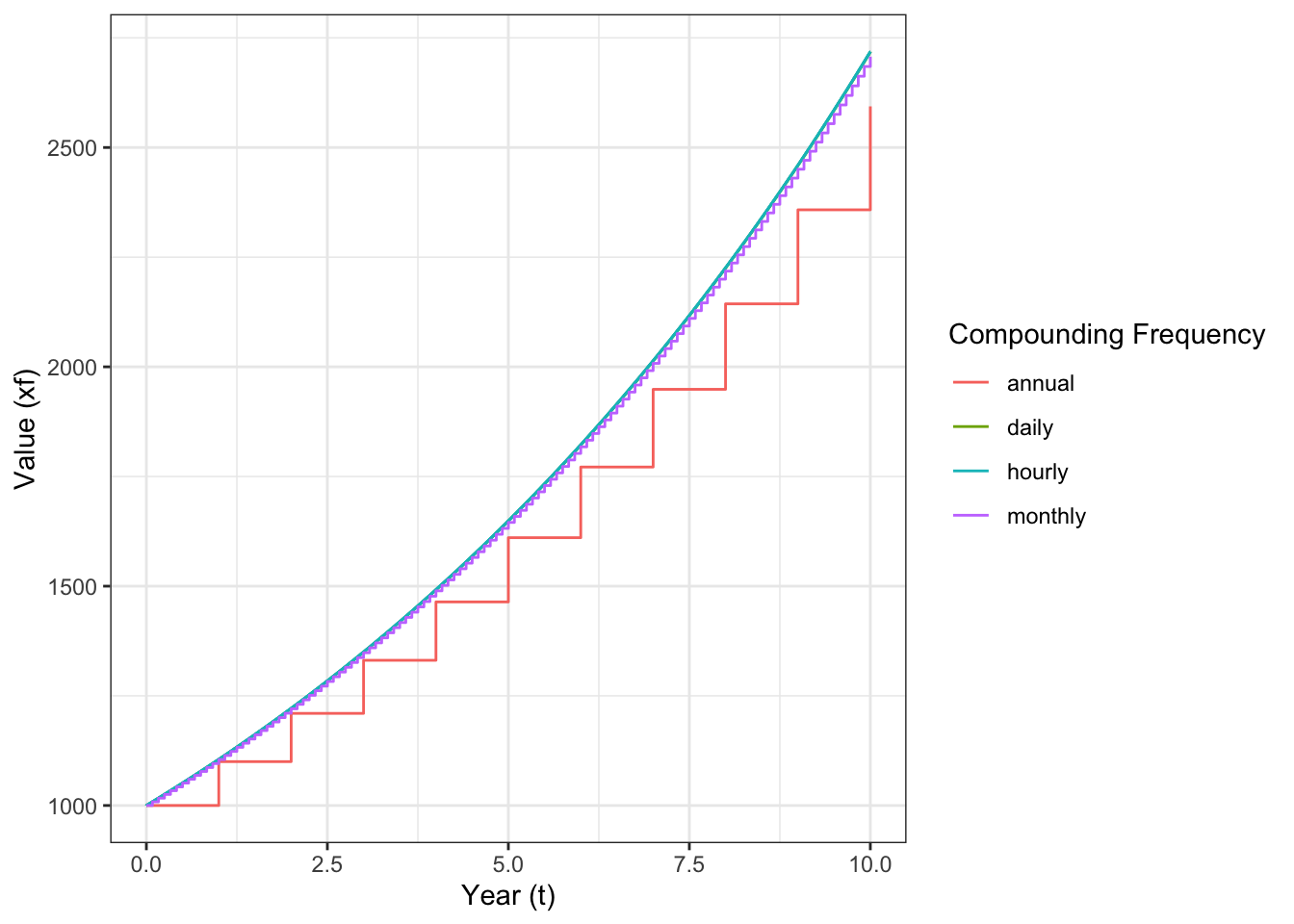
Figure 3.1: Growth of loan value at different compounding frequencies.

It turns out that if you take the limit $\lim_{k\to\infty} F=P[1+(i/k)]^{nk}$ you can derive the equation for continuously compounding interest,

\[\begin{equation} F=Pe^{in} \tag{3.2} \end{equation}\]

Using our new equation, we can find out how much money we will have after 10 years of continuously compounding the interest from our $1,000 invested at an interest rate of 10%.

Continuously: $\$1000*e^{(0.1*10)}=\$2718.28$

Notice that this value isn’t significantly more than the amount of interest earned by compounding the interest daily. As the number of compounding periods continues to increase, the interest earned in each period increases by a diminishing amount. However, remember that even when the difference may be small, the more frequent the compounding period, the more interest is generated.

3.2 Cash Flows

Now that we have a basic understanding of the time value of money and the power of interest, we can discuss some of the tools that are often used to finance projects. These financial tools are based on the time value of money, and work by using the power of interest to raise the funding necessary for projects.

Financial tools differ based on how the loan is structured (interest, compounding), whether the project can bring in revenue while it operates, and when and how the loan is paid off. Each of these variables can be difficult to describe. A cash flow diagram is a chart that shows inflows and outflows of cash over time for a project or company, and can be a way to simplify these complex exchanges.

First, imagine that you have taken out a student loan of $10,000 at a 5% interest rate. You want to pay this back over the next 10 years, so you decide to pay it off by putting $1250 towards the loan every year until the final year, when you will pay it off in full. This cash flow can be represented with the diagram in Figure 3.2.

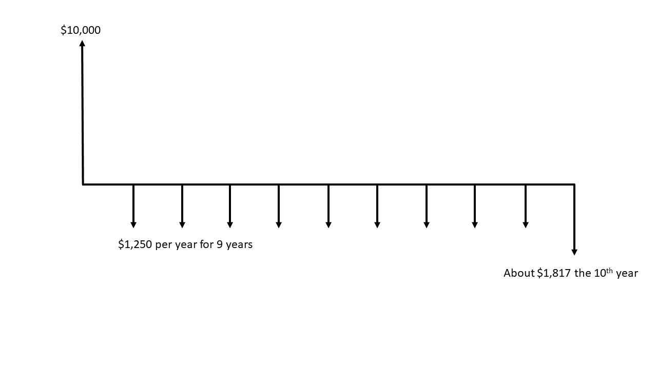
Figure 3.2: Cash flow diagram for a student loan and repayment.

The diagram is set up by drawing a horizontal line representing the time over which the cash flow takes place. Intervals represent periods of time, in this case years, starting at 0 when you initially borrow the $10,000. Arrows that point up show cash inflows, like the $10,000 you borrowed initially. Arrows that point down show cash outflows, like the payments you make over the next 10 years to pay back the loan. Notice that larger amounts have larger arrows, although they don’t need to be exactly proportional. Another important point is that each arrow represents the net cash flow for each period of time. In some cash flow diagrams you may have inflows and outflows during the same period, but they can be added together and represented using just one arrow.

Note that the borrower and the lender will each have their own cash flow diagram, and that these diagrams will be symmetrical. Let’s look at a couple of examples of cash flow diagrams. Let’s look at the diagram for the bank that loaned you the $10,000, shown in Figure 3.3. Because they lent the money, their cash flow diagram will be the opposite of yours.

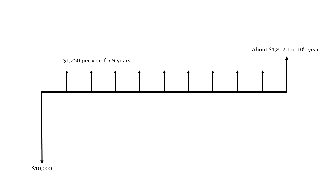
Figure 3.3: Cash flow diagram for a student loan and repayment; lender’s perspective.

These are simple cash flow diagrams. It is possible to represent complicated funding and revenue schemes with cash flow diagrams.

3.2.1 Financial Tools

Three basic tools¹⁰ are used to finance projects: mortgages, bonds, and sinking funds. We will discuss each of these in turn.

3.2.1.1 Mortgages

A mortgage is a loan for the purchase of property that uses the property as collateral. A bank or other investor gives a person or a company money to purchase a property (often a home). The property owner then makes regular payments to the bank to pay back the principal on the loan as well as the accumulated interest. If the owner is unable to make these payments, the bank can cancel the mortgage, seize the property, and resell the property to cover its losses. In the commercial world, mortgages allow the financing of large projects that would otherwise be too expensive to fund. They also allow people to buy houses that cost many times their annual salary and build real wealth.

Interest rates change for many reasons. Typically when the economy is doing well, interest rates rise to encourage people with money to invest it. When the economy is hurting, interest rates fall to encourage people to innovate or restructure their debts.¹¹ So it might happen at some point that a person could obtain a loan for an existing mortgage at a lower rate than they are currently paying. By refinancing, they can take out a second loan at a lower interest rate to pay off the original loan, and then continue paying off the new loan at the lower interest rate.

Making additional early payments on a mortgage can save substantial amounts of money later, depending on the interest rate.

3.2.1.2 Bonds

Bonds are agreements where a private investor loans a sum of money to a company or a government, and the company pays this principal (called the face value) back at the end date of the bond. The borrower also agrees to make regular interest payments (called the coupon) to the bond holder until the bond’s end date.

It is possible for a bondholder to sell their bonds to other investors. This might be advantageous if interest rates increase, allowing an investor to buy bonds with higher payments. On the market, bonds can be described in two terms:

value: the present worth of all future bond payments, including the payback amount. This will not necessarily be the sale price of the bond, because other bonds on the market might have more or less of their value in the interest payments.
yield: the ratio of the annual interest payment to the bond price.

If an institution fails to pay its bondholders, the institution is considered in default, and the bondholders can force the institution into bankruptcy. Institutions that are more likely to default therefore must pay higher interest rates to attract investors, and institutions that are unlikely to default (like the United States Treasury) pay very low rates compared to their peers.

Bonds are an especially important way for governments to raise money from many investors. In the case of a mortgage, most banks have the capital necessary to issue loans for houses (even many houses). But it would be very difficult for a bank to gather enough money to make a loan that would build an interstate freeway. It would also be impossible for a bank to repossess the interstate if the Department of Transportation couldn’t pay back the loan. Hence the importance of trust.

A special kind of bond can happen when the infrastructure will generate revenue, such as for a toll road. In this case, the investors might buy a portion of the tolls collected from the facility in exchange for a lower interest payment or a lower payback amount.

In revenue-financed bonds for toll roads, the forecasts of traffic engineers play a critical role in helping investors to set the terms of the bond. What might happen if the traffic forecasts are wrong?

3.2.1.3 Sinking Funds

Sinking funds are used to put aside money for a future expense. A company often creates a sinking fund for the payment of bonds, or for the eventual repayment of a large debt. Sinking funds can also be a powerful tool in individual retirement. By setting aside a set amount of money every month, a person can eventually create a large sum of money that will gain enough interest to pay their living expenses and allow them to retire. Letting time and interest work for you and investing now is much efficient than trying to save in the future.

The United States Highway Trust Fund was originally created as a sinking fund. Gasoline tax revenues would fill the fund, and transportation infrastructure projects would be paid from the interest on the fund. Unfortunately, the federal gasoline tax was set at a particular level (18.4 cents per gallon in 1993) and was not indexed to inflation or any other metric. Politicians in both major parties have resisted raising the gasoline tax in the last 30 years. This means that the purchasing power of the gas tax revenues have eroded from inflation even while increasing fuel efficiency lowers revenue per vehicle mile and construction prices have increased. The Highway Trust Fund now operates more like a dedicated budget, with Congress periodically needing to appropriate funds from other sources to pay for highway and transit infrastructure.

Is the current state of the Highway Trust Fund sustainable? Is that a problem? If not, what would be needed to make it sustainable?

3.3 Equivalence

Equation (3.1) introduced the idea that the future value of money $F$ is different than its present value after interest and time have been considered. We can turn this equation around to get the present value of future money as well:

\[\begin{equation} P=F(1+i)^{-n} \tag{3.3} \end{equation}\]

This is powerful because it allows us to translate complex cash flows defined with different interest rates and time frames into an equivalent present value.

Besides future and present values, two additional values might play a role in financial project planning and consideration. The first of these values is the annuity, $A$. This is the equal periodic payment that will repay a loan over time, or the equal period revenue expected from an investment. If we pay it all off in one period, then $F = A$. If it takes two periods, then the equation is $F = A + A*(1 + i)$ including interest paid in the second period. Extending the full series $n$ times and solving for $A$,

\[\begin{align} F &= A + A*(1 + i) + A* (1 + i)^2 + \ldots + A*(i+1)^{n-1} = \sum_{j = 0}^{n -1} A ( 1 + i)^j\\ F(1 + i) &= \sum_{j = 1}^n A ( 1 + i)^j \\ F(1 + i) - F &= \sum_{j = 1}^{n } A ( 1 + i)^j - \sum_{j = 0}^{n-1} A ( 1 + i)^j \\ F+ Fi - F &= A*(1 + i)^n - A\\ Fi &= A*[(1 + i)^n - 1]\\ F &= A*\frac{(1 + i)^n - 1}{i} \tag{3.4} \end{align}\]

To turn a future value into an equivalent annuity, we just take the inverse.

\[\begin{equation} A=F*\frac{i}{(1+i)^{n}-1} \tag{3.5} \end{equation}\]

We could also derive equivalence between the annuity and its present value.

\[\begin{equation} P=A*\frac{(1 + i)^n -1}{i (1 + i)^n} \tag{3.6} \end{equation}\]

\[\begin{equation} A=P*\frac{i ( 1 + i) ^n}{(1 + i)^n - 1} \tag{3.7} \end{equation}\]

Assume that you are purchasing a home worth $200k with no down payment. The interest on the loan compounds annually at 4% interest and has a 30-year term. What is the monthly payment on the mortgage? How much will you pay on the home in total? What is the equivalent value of that money at the end of the mortgage.

We calculate the monthly payment as an annuity given a present value. So Using Equation (3.7),

\[\begin{align*} A &=200000*\frac{0.04(1+0.04)^{30}}{(1+0.04)^{30}-1}\\ A &= 11,566 \quad\textrm{per year}/12\\ A &= 964 \quad\textrm{per month} \end{align*}\]

The total amount paid is the sum of all annuities, or $346,981. The actual value of that amount is the future value of the annuity, or

\[\begin{align*} F &= 11,566 *\frac{(1+0.04)^{30}-1}{0.04}\\ F &= 648,680 \end{align*}\]

The second value is a gradient, or an annuity that increases its value over time by a uniform amount $G$¹². That is if $G = 100$, then $G_1 = 100, G_2 = 200, \ldots, G_n = n*G$. This can happen if, for instance, you expect that a business in operation will grow in each period, or if you plan to pay a larger amount on your mortgage as your income increases. We won’t do the derivation of this value, but the equations are:

\[\begin{equation} P=G*\left[\frac{(1+i)^{n}-1}{i^2(1+i)^{n}}-\frac{n}{i(1 + i)^n}\right] \tag{3.8} \end{equation}\]

\[\begin{equation} F=G*\left[\frac{(1+i)^{n}-1}{i^2}-\frac{n}{i}\right] \tag{3.9} \end{equation}\]

\[\begin{equation} A=G*\left[\frac{1}{i}-\frac{n}{(1+i)^n-1}\right] \tag{3.10} \end{equation}\]

Maintenance on an old machine is $100 this year but is expected to increase by $25 each year thereafter. What is the present worth of five years of maintenance? Assume an interest rate of 10%.

This is an interesting problem because it involves both an annuity ($100 per year) and a gradient of $25 each year. The cash flow diagram looks like this:

We can then calculate the present value of each element separately and add them together,

\[\begin{align*} P&=G*\left[\frac{(1+i)^{n}-1}{i^2(1+i)^{n}}-\frac{n}{i(1+i)^{n}}\right]\\ &=25*\left[\frac{(1+0.1)^{5}-1}{(0.1)^2(1+0.1)^{5}}-\frac{5}{0.1(1+0.1)^{5}}\right]\\ &=172\\ P&=A*\frac{(1+i)^{n}-1}{i(1+i)^{n}}\\ &=100*\frac{(1+0.1)^{5}-1}{0.1(1+0.1)^{5}}\\ &=379 \end{align*}\]

for a total present value of $551

In all of our equivalence equations to this point, we necessarily assume some end-point $n$ time periods in the future. But what about the equivalent present value of a perpetual benefit? This often occurs when considering the worth of capital investments; if we want to find the present worth of this endless series of payments, we can use a simple formula for capital worth

\[\begin{equation} P=\frac{A}{i} \tag{3.11} \end{equation}\]

3.3.1 Calculation Shortcuts

It is important to know that the equations we have discussed so far exist, and that they are not magical constructs banks designed to part you from your money. But the equations themselves are somewhat unwieldy and impractical, and they are certainly difficult to remember. There are two primary shortcuts that you should be aware of.

Preexisting or custom software functions
Factor tables

3.3.1.1 Functions

In practice, you will probably use functions that pre-exist in Excel or that you code yourself into software that you write. The examples on this page use functions that I wrote in the R programming language. For example, we can write a function for Equation (3.1) that converts P to F, and then use that function to quickly find the future value for each of the compounding rates in the the example above:

# function to find F given P, i, n, k
ptof <- function(P, i, n, k){
  P * (1 + (i / k) )^(n * k)
}
# 1000 for ten years at 10%, compounding at different rates
for(k in c(1, 12, 365, 365 * 24)) {
  print(ptof(1000, 0.1, 10, k))
}

## [1] 2593.742
## [1] 2707.041
## [1] 2717.91
## [1] 2718.266

In Excel, there are an array of functions that you can use. For example, the FV() function will compute the future value of an investment given either an initial value or a regular payment. That means, the FV function works both as Equation (3.1) and also as Equation (3.4). The results and use of this function are shown in Figure 3.4.

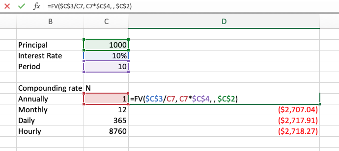
Figure 3.4: Excel FV function in use.

3.3.1.2 Factor Tables

On the FE exam and the exams in this class, you will not have access to Excel or to a programmable calculator. It is impractical to type in every element of each formula repeatedly; you are bound to make several mistakes.

Notice though that each equation we have looked at is the product of a scalar ($A$, $F$, etc.) and some factor of the interest rate and the time period. Watch what happens when we take a set of present values increasing by factors of 10 at a constant interest rate and time period.

for(P in c(1, 10, 100)){
  print(ptof(P, 0.1, 1, 10))
}

## [1] 1.104622
## [1] 11.04622
## [1] 110.4622

Unsurprisingly, the future values are direct multiples of the present value. This means we could create a table that contains the factors for different interest rates and periods. A table for 2% interest is in Table 3.1. The way to read these tables is as follows:

Identify the table for the interest rate you are given.
Determine which column of factors you need. You read $F/P$ as “$F$ given $P$”, so this is your column if you have been given a present value and wish to find the future value.¹³
Find the row in the table for the given number of periods. If $F/P$ is your column and the number of time increments is 5, your value is 1.1041.
Multiply the original given value by the value from the table. Keeping with the same example, if you were given 1,000 dollars for $P$, you multiply it by 1.1041 to find $F$ = 1,104.10 dollars.

Table 3.1: Factor Table: i = 2.00%
n	P/F	P/A	P/G	F/P	F/A	A/P	A/F	A/G
1	0.9804	0.9804	0.0000	1.0200	1.0000	1.0200	1.0000	0.0000
2	0.9612	1.9416	0.9612	1.0404	2.0200	0.5150	0.4950	0.4950
3	0.9423	2.8839	2.8458	1.0612	3.0604	0.3468	0.3268	0.9868
4	0.9238	3.8077	5.6173	1.0824	4.1216	0.2626	0.2426	1.4752
5	0.9057	4.7135	9.2403	1.1041	5.2040	0.2122	0.1922	1.9604
6	0.8880	5.6014	13.6801	1.1262	6.3081	0.1785	0.1585	2.4423
7	0.8706	6.4720	18.9035	1.1487	7.4343	0.1545	0.1345	2.9208
8	0.8535	7.3255	24.8779	1.1717	8.5830	0.1365	0.1165	3.3961
9	0.8368	8.1622	31.5720	1.1951	9.7546	0.1225	0.1025	3.8681
10	0.8203	8.9826	38.9551	1.2190	10.9497	0.1113	0.0913	4.3367
11	0.8043	9.7868	46.9977	1.2434	12.1687	0.1022	0.0822	4.8021
12	0.7885	10.5753	55.6712	1.2682	13.4121	0.0946	0.0746	5.2642
13	0.7730	11.3484	64.9475	1.2936	14.6803	0.0881	0.0681	5.7231
14	0.7579	12.1062	74.7999	1.3195	15.9739	0.0826	0.0626	6.1786
15	0.7430	12.8493	85.2021	1.3459	17.2934	0.0778	0.0578	6.6309
16	0.7284	13.5777	96.1288	1.3728	18.6393	0.0737	0.0537	7.0799
17	0.7142	14.2919	107.5554	1.4002	20.0121	0.0700	0.0500	7.5256
18	0.7002	14.9920	119.4581	1.4282	21.4123	0.0667	0.0467	7.9681
19	0.6864	15.6785	131.8139	1.4568	22.8406	0.0638	0.0438	8.4073
20	0.6730	16.3514	144.6003	1.4859	24.2974	0.0612	0.0412	8.8433
21	0.6598	17.0112	157.7959	1.5157	25.7833	0.0588	0.0388	9.2760
22	0.6468	17.6580	171.3795	1.5460	27.2990	0.0566	0.0366	9.7055
23	0.6342	18.2922	185.3309	1.5769	28.8450	0.0547	0.0347	10.1317
24	0.6217	18.9139	199.6305	1.6084	30.4219	0.0529	0.0329	10.5547
25	0.6095	19.5235	214.2592	1.6406	32.0303	0.0512	0.0312	10.9745
30	0.5521	22.3965	291.7164	1.8114	40.5681	0.0446	0.0246	13.0251
40	0.4529	27.3555	461.9931	2.2080	60.4020	0.0366	0.0166	16.8885
50	0.3715	31.4236	642.3606	2.6916	84.5794	0.0318	0.0118	20.4420
60	0.3048	34.7609	823.6975	3.2810	114.0515	0.0288	0.0088	23.6961
100	0.1380	43.0984	1464.7527	7.2446	312.2323	0.0232	0.0032	33.9863

You will need $10,000 in 5 years, and you can invest at 2% interest. How much do you invest now? How much would you invest each year?

You wish to find the present value given a future value, so you want the $P/F$ column. The factor for this column in the 2% table at 5 years is 0.906, so you have \[\begin{align*} P &= F * P/F(0.02, 5)\\ P &= 10,000 * 0.906\\ &= 9,057\\ \end{align*}\]

The second half of the question asks us to find the equivalent annuity given a future value, so we look up the $A/F$ factor, which is 0.192.

\[\begin{align*} A &= F * A/F(0.02, 5)\\ A &= 10,000 * 0.192\\ &= 1,922\\ \end{align*}\]

3.4 Returns

The reason to undertake projects is to receive a return of benefits. If you are a developer, you want to build something that will generate income justifying the cost of construction. If you are building public infrastructure, the benefits might not be economic (although they could be). From the investor side, you want lend your money to a project that has the highest expected revenue, considering risk.

3.4.1 Net Present Value

With the help of the equivalence equations we learned in the previous section, we can find the net present value (NPV) of a project, or the current value of all future cash flows. If the NPV is positive, then the project will result in a positive return on investment. If it is negative, then the project will lose money over its life. An equation for the NPV is

\[\begin{equation} NPV=\sum_{t=0}^{n} \frac{R_t}{(1+i)^t} \tag{3.12} \end{equation}\]

$R_t$: net cash flow for a given time t
$i$: interest / discount rate
$t$: period of time

Note that the $R_t/(1+i)^t$ is the same as $P/F(i, t)$, or the equivalence function to bring a future value to the present.

Consider a project with the following projected cash flow¹⁴, shown with its present value assuming a discount rate of 10%. What is the NPV of the project?

Table 3.2: Example Cash Flow
t	invested	earned	pv_invested	pv_earned
1	1000	0	909.0909	0.00000
2	1000	100	826.4463	82.64463
3	0	200	0.0000	150.26296
4	0	400	0.0000	273.20538
5	0	600	0.0000	372.55279
6	0	600	0.0000	338.68436
7	0	600	0.0000	307.89487
8	0	500	0.0000	233.25369
9	0	300	0.0000	127.22929
10	0	100	0.0000	38.55433
total	2000	3400	1735.5372	1924.28230

The NPV is the difference between the present value of all earnings and the present value of all investments, which in this case is

\[\begin{align*} NPV &= 1,924 - 1,736\\ &= 189\\ \end{align*}\]

How much the project gains or loses is an important consideration beyond the binary win / lose scenario: every investment has an opportunity cost. If I invest in one project, I cannot invest in another. So we need some way to determine what the return is. I should look for investments that maximize my return. One method is the annual return on investment, which is the ratio of the present annual revenue $P_{e}/n$ relative to the total investment $I$,

\[\begin{equation} ROI_t = \frac{P_{e}/n}{I} \tag{3.13} \end{equation}\]

What is the ROI implied in the previous example?

The developer receives a present value annuity of $192 (this is found by dividing the pv_earned total by the number of years) over the ten-year life of the project as a return on their $1,736 investment. Using (3.13),

\[\begin{align*} ROI_t &= \frac{P_{e}/n}{I}\\ &= \frac{192}{1,736}\\ &= 0.111 \end{align*}\] or a 11.1% equivalent annual ROI.

Note that the ROI depends on the discount rate. If the discount rate were higher, the present value of the expected earnings would be reduced, leading to a change in the NPV.

Consider a project with the same projected cash flow, but with a discount rate of 13%. What is the NPV and ROI of the project?

t	invested	earned	pv_invested	pv_earned
1	1000	0	884.9558	0.00000
2	1000	100	783.1467	78.31467
3	0	200	0.0000	138.61003
4	0	400	0.0000	245.32749
5	0	600	0.0000	325.65596
6	0	600	0.0000	288.19112
7	0	600	0.0000	255.03639
8	0	500	0.0000	188.07993
9	0	300	0.0000	99.86545
10	0	100	0.0000	29.45883
total	2000	3400	1668.1024	1648.53987

The NPV is $-19.6 and the ROI is 9.88%

3.4.2 Setting the MARR

This brings up the question of what discount rate should be used, and how this discount rate is determined. Recall that the discount rate has to account for:

Risk: when you lend money, it might not always come back
Inflation: money will be worth less in the future
Opportunity Cost: you might be able to do something else with your money

In this way, the discount rate represents a Mimumum Acceptable Rate of Return (MARR). If a project’s returns are lower than the combined risk, inflation, and opportunity cost, then it is not a smart investment.

In the previous examples, the interest rate was set first at 10%, and then at 13%. If these numbers represent the MARR for the investor, is the project a wise investment?

At 10%, we calculated the ROI as 11.1%, which exceeds the MARR. But at 13%, the ROI was only 9.88%, meaning that it would not be a good investment.

Every actor in an economy including business owners, developers, investors, and individuals will have their own MARR when evaluating a project. Let’s unbundle the three elements of the discount rate: \[\begin{equation*} F = P*(1 + \text{risk})^n(1 + \text{inf} )^n(1 + \text{opp.cost})^n \end{equation*}\]

Because each of these rates individually is small (somewhere less than 10%), we can simplify this to a single rate that includes all three elements, \[\begin{equation} F \approx P(1 + \text{risk} + \text{inf} + \text{opp.cost})^n \tag{3.14} \end{equation}\] We can also make this assertion because each element of $i$ cannot really be definitively known. Having said that, there are reference points that can be used for these values. Governments regularly publish inflation statistics; using the long-run or recent short-run average inflation rate could be a good benchmark depending on the application. Further, government bonds for stable countries are seen as relatively risk-free investments; at the very least, the MARR for an investor should exceed the interest paid on those bonds. Finally, the market can show what investors are currently paying for bonds of equivalent risk.

Your company plans to sell bonds to investors to raise revenue for a project. U.S. Treasury bonds have been recently selling at 5% interest, and are perceived to be a risk-free investment. A company with a similar risk profile recently sold bonds at 8% interest, but inflation forecasts have increased from 1% to 3%. How much interest should your company expect to pay on these bonds?

The MARR should include each element, but it is important to remember that the U.S. Treasury bonds already account for the existing inflation. Also, the interest paid by the reference company includes the opportunity cost, risk, and previous inflation forecast. So the MARR for investors is:

5% opportunity cost and baked-in inflation
3%-1% = 2% new inflation forecast
8% - 5% = 3% risk relative to treasuries

Your company should expect to pay 10% interest on your bonds, because that will be the MARR of your investors.

When a company is considering the MARR for its own projects, it has a different opportunity cost. When raising money, a company may sell stocks in itself in exchange for a share of its future profits. If there is nothing else to spend money on, the company could always buy its shares back and therefore keep more of its profits. The rate at which a company can make this conversion is called the weighted average cost of capital (WACC). Its MARR should therefore be at least this value. Of course, a company will not pursue every project with an ROI greater than its WACC, because doing so might expose the company to lots of risk, which would raise the MARR for investors that might buy the company’s stock. A company might set its MARR differently for projects of different sizes, with differing ranking and selecting criteria.

For an individual, the MARR should reflect inflation, risk, and the time that could be spent working on something else. In a very real sense, MARR is subjective.

3.4.3 Internal and External Rates of Return

One serious problem with using ROI as a project comparison tool is that the ROI as we’ve looked at it to this point depends heavily on the asserted or assumed discount rate. another potential option is the internal rate of return. This is the discount rate at which the NPV of the project is zero, or at which the present value of all cash flows is zero.

Using the cash flow from the returns example, find the internal rate of return.

We can use Excel’s Goal Seek function to find that the NPV of the project is zero at a discount rate of 12.69%

Table 3.3: Example Cash Flow at IRR
t	invested	earned	pv_invested	pv_earned
1	1000	0	887.3902	0.00000
2	1000	100	787.4613	78.74613
3	0	200	0.0000	139.75709
4	0	400	0.0000	248.03815
5	0	600	0.0000	330.15992
6	0	600	0.0000	292.98068
7	0	600	0.0000	259.98818
8	0	500	0.0000	192.25913
9	0	300	0.0000	102.36532
10	0	100	0.0000	30.27933
total	2000	3400	1674.8515	1674.57393

The IRR has the advantage of not relying on an assumed discount rate. However, it also has a weakness in that under certain circumstances, the IRR for a given cash flow is not unique; e.g., a complicated cash flow might show a zero NPV at 2% and at 9%. To get around this, we can consider the external rate of return, which is the rate at which the future value of earning periods equal the grown present value of the investments, or $e$ in the equation

\[\begin{equation} F_E= P_I(1 + e)^n \tag{3.15} \end{equation}\]

To calculate the ERR:

Calculate the net cash flow in each period.
Discount all negative periods to their present value using an assumed rate.
Grow all positive periods to their future value using an assumed rate.
Calculate the rate necessary to grow the present value of losses to the future value of earnings.

Of course, finding the ERR requires an assumed discount rate, putting us in the same position as before.

Using the same cash flow, find the external rate of return assuming a discount rate of 10%.

The table below shows the present value of the losses and the future value of the earnings for each period using a discount rate of 10%. We now want to find $e$ such that

\[\begin{align*} F_E &= P_I(1 + e)^n\\ 4776.73 &= 1652.89(1 + e)^{10}\\ e&= 11.196\% \end{align*}\]

Table 3.4: Example Cash Flow to find ERR
t	invested	earned	net	pv_invested	fv_earned
1	1000	0	-1000	-909.0909	0.0000
2	1000	100	-900	-743.8017	0.0000
3	0	200	200	0.0000	389.7434
4	0	400	400	0.0000	708.6244
5	0	600	600	0.0000	966.3060
6	0	600	600	0.0000	878.4600
7	0	600	600	0.0000	798.6000
8	0	500	500	0.0000	605.0000
9	0	300	300	0.0000	330.0000
10	0	100	100	0.0000	100.0000
total	2000	3400	NA	-1652.8926	4776.7338

3.5 Project Assessment

In the previous section on returns, we looked at project evaluation largely as a binary consideration: is the ROI greater than the MARR? Or, is the NPV positive?

It is rare to only have one course of action in an investment. More typically, there are multiple different strategies or alternatives that you need weigh against each other. In this section, we will discuss how to comparatively evaluate projects with different timelines, discount rates, and other variables.

3.5.1 NPV and ROI

NPV and ROI are convenient methods to compare projects. These measures can sometimes identify different preferred alternatives, however.

Four different alternative highway maintenance regimens — plus a “do-nothing” alternative — are being considered. The present value of the long-run benefits (earnings) and costs (investments) are given in the table below. Calculate the NPV and ROI for each alternative. Assume a discount rate of 8%.

We can calculate the ROI for the highway maintenance example by first converting the NPV of the benefits into a perpetual annualized rate using Equation (3.11). The ROI for alternative $A$ is therefore $24 * 0.08 / 7 = 27.43$. The NPV for alternative $A$ is simply $24-7 = 17$ For all options,

Alternative	Benefit	Cost	ROI	NPV
Do Nothing	0	2	0.00	-2
A	24	7	27.43	17
B	11	9	9.78	2
C	41	17	19.29	24
D	43	32	10.75	11

Based on ROI, the preferred alternative is $A$, but based on NPV the preferred alternative is $C$.

3.5.2 Benefit / Cost

In the previous section, we calculated ROI as the ratio of the annualized benefits to the total investment. We could also compute the simple ratio of benefits to costs as a rudimentary measure. If the ratio $B/C > 1$, then the project is feasible. If a project has a higher $B/C$ ratio, it could be more attractive.

The present value of benefits and costs of four alternative highway maintenance projects (plus a “do nothing” alternative) are given below.¹⁵ Calculate the $B/C$ ratio.

Alternative	Benefit	Cost	B/C
Do Nothing	0	2	0.00
A	24	7	3.43
B	11	9	1.22
C	41	17	2.41
D	43	32	1.34

By this measure, alternative $A$ is the best option.

But a simple ratio does not explain everything. What if a project has substantially more benefits but also more costs? What might be desirable is an incremental benefit / cost analysis. In this case, we could calculate the marginal $B/C$ ratio between pairs of alternatives,

\[\begin{equation} B/C_{b-a} = \frac{B_b - B_a}{C_b - C_a} \tag{3.16} \end{equation}\]

If the incremental $B/C$ is greater than one, it is an indication that the benefits exceed the costs relative to the previous alternative. To find the most efficient alternative, do the following:

Order the alternatives by cost.
Compute the incremental $B/C$ ratio between successive alternatives.
For each successive alternative, reject or accept the new alternative based on whether the new $B/C$ ratio is greater than one.

It can also be really helpful to graph the benefits versus costs on a graph, to see where the marginal increase in benefit versus the marginal increase in costs starts to turn. The slope of the line between alternatives on the upper edge of the plot is the incremental $B/C$ between those alternatives. The most efficient alternative is the last one with an incremental slope greater than 1.

For the highway maintenance projects considered previously, what is the preferred alternative in terms of relative efficiency?

The costs of the alternatives are already in the correct order. We can therefore calculate the incremental benefit to cost ratio between each successive project.

Alternative	Benefit	Cost	Incremental benefit	Incremental cost	Inc. B/C	Decision
Do Nothing	0	2	0	0	NaN	Base
A	24	7	24	5	4.80	Accept A over Do Nothing
B	11	9	-13	2	-6.50	Reject B, Keep A
C	41	17	17	10	1.70	Accept C over A
D	43	32	2	15	0.13	Reject D, Keep C

Plotting the benefits and costs of each alternative helps us to visualize the incremental $B/C$ ratios.

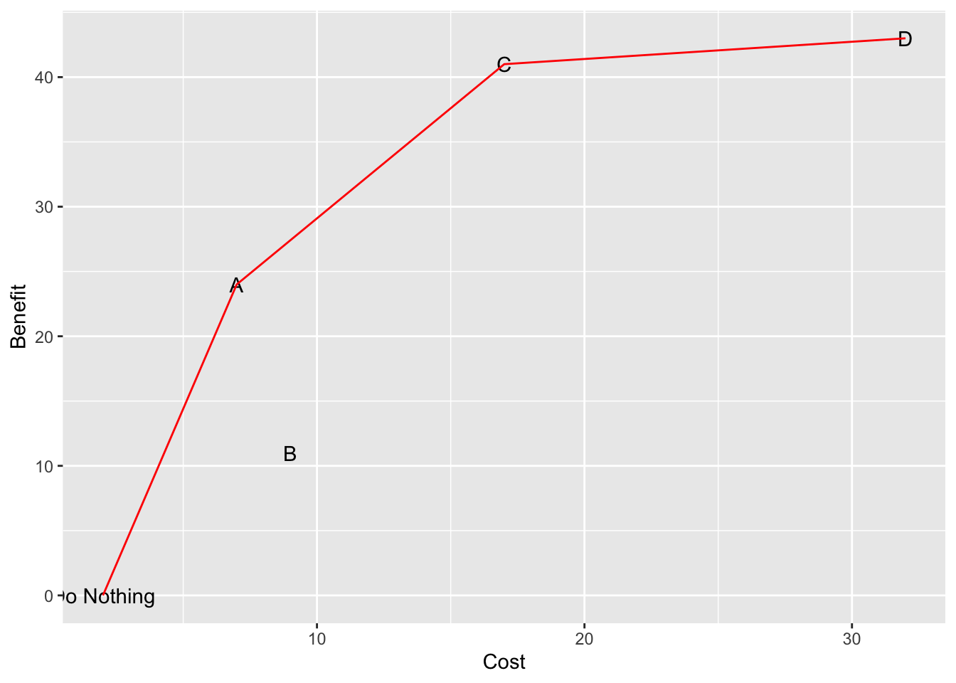
It is clear that alternative $B$ delivers substantially fewer benefits at a higher cost than $A$. Alternative $C$ provides more benefits than $A$, but at a higher cost. The incremental analysis suggests that this alternative is more efficient overall. The marginal benefits of alternative $D$ relative to alternative $C$ are not as impressive given the large cost increase of moving from $C$ to $D$.

It should be added that public projects often use $B/C$ ratios, and private projects often will use ROI or internal rate of return to select between alternatives. But usually, large civil infrastructure projects need to consider much more than simple benefit / cost ratios.

3.5.3 Evaluation Matrices

Many large public projects have benefits and costs that occur on a wide spectrum of different dimensions. There is the triple-bottom line discussed in Chapter1, but within each of these dimensions can be multiple different variables that require consideration. A common method to put these variables on equal footing is with an alternatives evaluation matrix. To create this matrix:

Decide which elements of a project, in terms of benefits and costs or other outcomes need to be considered. This may involve public input.
Develop a scoring system $b$ for each element. This is often a score of 1 to 5 or a grade of A to F or some other categorical measure.
Develop weights $w$ for each element, again with public input.
Calculate the weighted score of each alternative as $S_a= \sum_e w_e*b_{ea}$ where $S$ is the total weighted score for the alternative, $w_e$ is the weight of each element $e$, and $b$ is the score of within that element for each alternative.

Figure 3.5 shows a project evaluation matrix from the Utah Transit Authority’s Point of the Mountain alternatives analysis. UTA has developed five different alternatives to provide high-frequency transit to Lehi and the site currently occupied by the Utah State Prison, using different combinations of light rail extensions and new BRT service. These five alternatives are each evaluated on a five-point scale applied to 19 different measures grouped into five general categories:

Transit System Performance
Access and Mobility
Land Use
Cost and Constructability
Natural and Built Environment

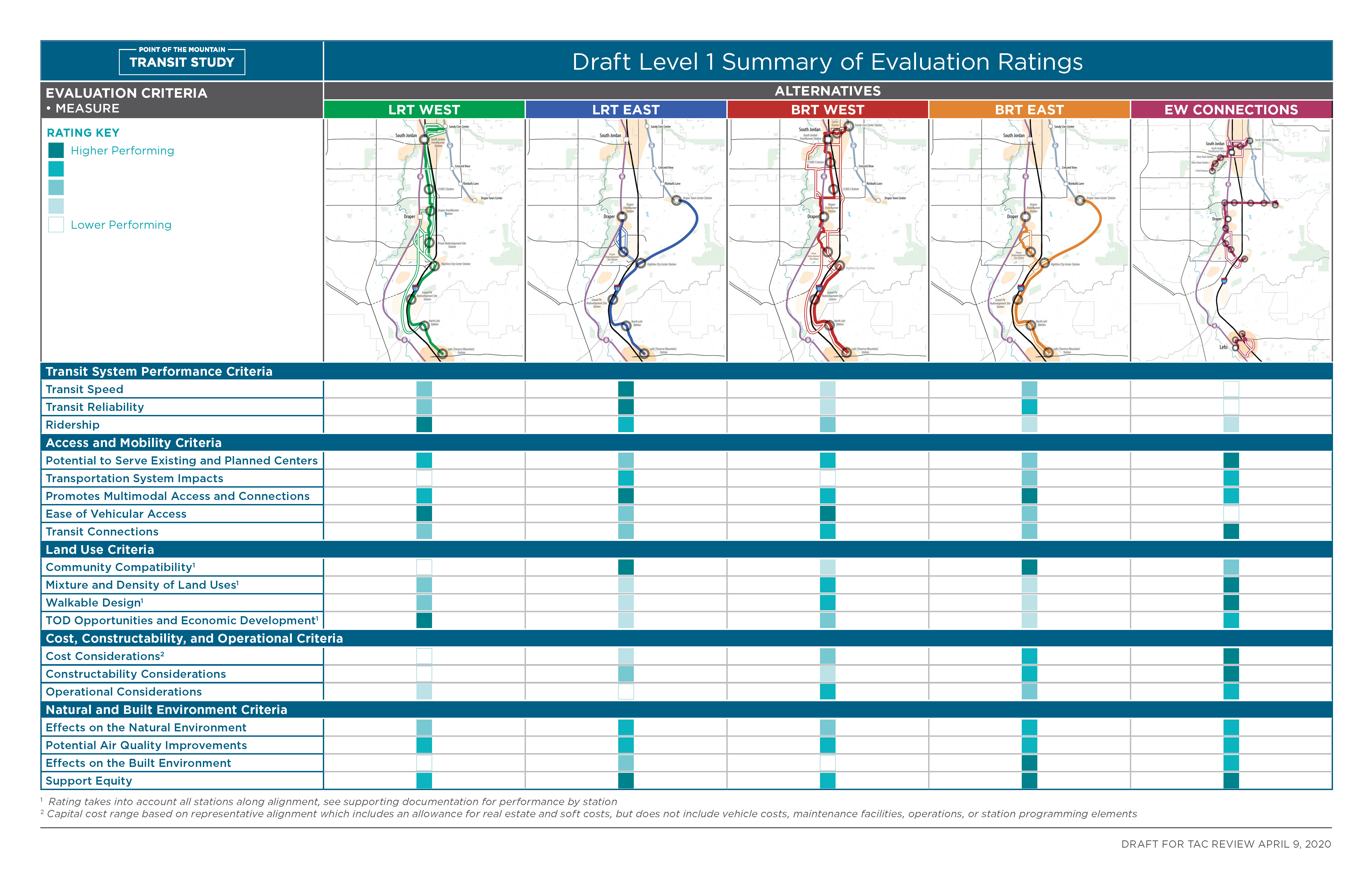
Figure 3.5: Point of the Mountain Transit Study alternatives analysis.

You can see in the figure how each alternative generally performs. The EW Connections alternative scores the best in terms of cost, but it performs poorly in terms of transit speed and reliability. The LRT East and BRT East alternatives have similar profiles, but the BRT option trades a bit of speed and reliability for a lower cost.

When conducted in this way, a number of different factors besides pure cost and benefit are allowed to contribute to the overall project evaluation. There is also a risk, however, that this method can become purely subjective if care is not taken to avoid pre-determining the outcome.

3.6 Rules and Regulations

In this section, we discuss a series of issues related to how project evaluation interacts with public policy and other laws.

3.6.1 Taxes and Depreciation

Businesses pay taxes, though the specific amount of taxes paid depends greatly on how a business is structured, the specific industry it is working in, and how its profits are reinvested. If a business reinvests all its profits or claims a loss in a year, it is not uncommon for the business to pay little or no taxes. In general, the effective tax rate the business pays affects its MARR: if tax rates are high, then the MARR will have to be commensurately high and many otherwise viable projects will not be pursued.

Tax policy becomes an especially important issue when considering capital expenditures. Often, a business will invest a substantial amount of money to construct a building or purchase a piece of machinery. When the business is finished with the asset, it will sell or salvage the asset for its remaining value. The cash flow diagram for this transaction is as follows:

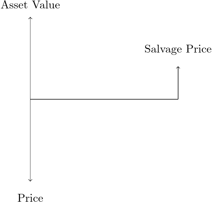
This has important ramifications for the taxes paid by the firm. When purchased, the expense was simply converted into an asset. But when the business sells the asset, it must pay taxes on the salvage value, even though the asset has lost much of its value. Accounting practice — and defined under tax law — is to consider the the depreciation of capital value as a business expense. There are many ways to calculate this, but we will focus on two: straight-line depreciation and the Modified Accelerated Cost Recovery System (MACRS).

In straight-line depreciation, the asset is assumed to lose its value at a constant rate to its salvage value $n$ periods in the future. The depreciation expense in year $j$ is:

\[\begin{equation} D_j=\frac{C-S_n}{n} \tag{3.17} \end{equation}\]

Where

$D_j$: depreciation in year $j$
$C$: initial cost
$n$: expected life of asset
$S_n$: expected salvage value in year $n$

Your firm purchases a $50k truck and intends to use it for seven years, at which point you expect to sell the truck for $20k. What is the capital expense you would claim in each year?

The capital expense from depreciation in any year is simply

\[\begin{align*} D_j&=\frac{C-S_n}{n}\\ &=\frac{50,000-20,000}{7}\\ &=4,285.71 \end{align*}\]

There are two problems with straight-line depreciation. First, the salvage value must be known or assumed. This probably works well for commodity capital expenses like trucks and other common machinery. It may work less well for unique assets like buildings. The other problem is that many assets do not lose a constant value each year: trucks lose more value in their first year than they do in their fifth. The MACRS depreciation technique accounts for both of these limitations.

Using MACRS, there is an assumed recovery period, and the depreciation within a particular year $Dj$ is simply the initial cost multiplied by a factor,

\[\begin{equation} D_j=C\times M_{jn} \tag{3.18} \end{equation}\]

The MACRS factors are given in the table below.

MACRS FACTORS¹
Year (j)	Recovery Period (Years)
Year (j)	3	5	7	10
1	33.33	20	14.29	10.00
2	44.45	32	24.49	18.00
3	14.81	19.2	17.49	14.40
4	7.41	11.52	12.49	11.52
5		11.52	8.93	9.22
6		5.76	8.92	7.37
7			8.93	6.55
8			4.46	6.55
9				6.56
10				6.55
11				3.28
¹ Factors given as percent values.

Your firm purchases a $50k truck and intends to use it for seven years. What is the depreciation capital expense in year 3?

In the MACRS table, we see that the factor in year 3 of an asset with a 7-year recovery period is 17.49%. Therefore, $D_j = 50000 * 0.1749 = 8,745$

The book value of an asset is the initial cost minus cumulative depreciation:

\[\begin{equation} BV=C-\sum{D_j} \tag{3.19} \end{equation}\]

Note that the MACRS book value will not incorporate the salvage value into its evaluation. The book value is therefore is not the fair market value, or how much you would expect to be paid for the asset. Additionally, the book value of capital does not include the value of land, but only capital assets constructed on that land (because land value cannot be depreciated).

Your firm purchases a $50k truck and intends to use it for seven years, at which point it will have a salvage value of $20k. What is the book value in each year, calculated using straight-line depreciation and MACRS?

j	Straight Line Dj	Straight Line BV	MACRS Dj	MACRS BV
0	0.000	50000.00	7145	42855
1	4285.714	45714.29	12245	30610
2	4285.714	41428.57	8745	21865
3	4285.714	37142.86	6245	15620
4	4285.714	32857.14	4465	11155
5	4285.714	28571.43	4460	6695
6	4285.714	24285.71	4465	2230
7	4285.714	20000.00	2230	0

3.6.2 Zoning

Almost all cities in the United States have zoning laws that specify what kinds of projects can be built in which kinds of areas. Figure 3.6 shows the zones in central Provo (a complete map with legend is available from Provo City). Regulations often captured in zoning codes include:

Activities permitted on site; most businesses that attract customers or conduct manufacturing are not permitted in residential zones.
Building height and floor-area ratio: how large of a structure can be permitted on the lot relative to its size?
Minimum lot size: This larely applies in residential zones, where cities may desire a certain amount of density.
Setbacks: structures may not be built within a certain distance of property boundaries.

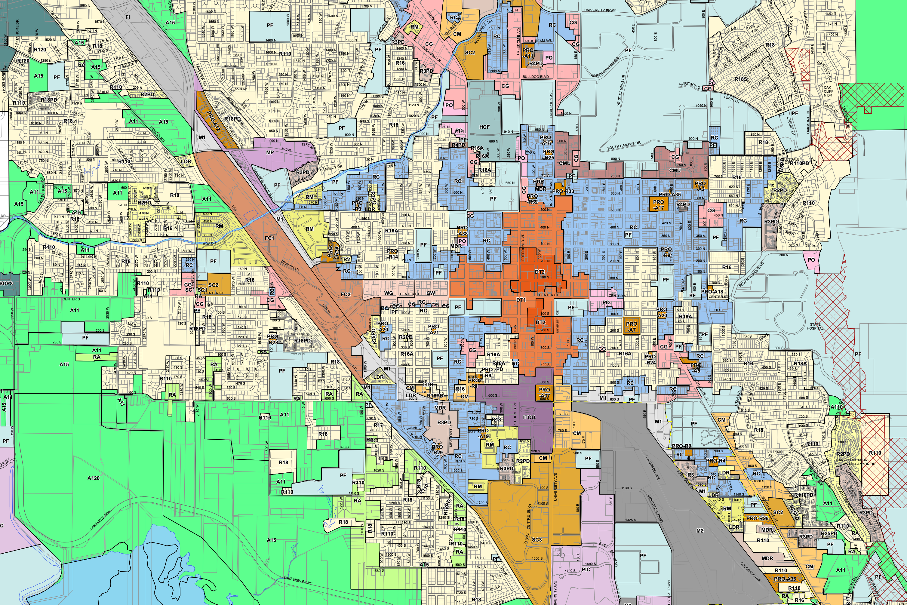
Figure 3.6: Zoning map in central Provo, Utah.

A developer might apply for a zoning variance or to have the property re-zoned. Changing a particular property from one zone to another zone may result in important benefits to the property owner, because the developer could put a larger and more profitable structure on the site. Variances and re-zonings are not uncommon, which is why zone maps can look so piecemeal. That said, these variances and zoning decisions can be politically contentious if local residents perceive the change in zoning as potentially harming their property values or neighborhood character.

Provo zoning codes prohibit renting homes in the Tree Streets and Edgemont neighborhoods near campus to more than one household, with certain exceptions. It is illegal, for instance, to rent a home to a family on the main floor and also rent to a group of single undergraduates in the basement.

What are the possible implications of this policy?

3.6.3 Environmental Impacts

The National Environmental Policy Act (NEPA) is a federal law that requires all federal agencies to evaluate the environmental consequences of their proposals prior to making decisions. This applies to direct actions by federal agencies, as well as indirect actions including all projects that use federal money — like most large civil infrastructure projects.

NEPA does not say that projects can have no environmental impact. It does say that the potential impacts must be known, and that an equivalent alternative with fewer environmental impacts could not be found. The process for ensuring that a project complies with NEPA is as follows:

The agency determines if the project falls under a Categorical Exclusion (CATEX). This happens when common projects have been previously determined to have no significant impact. If a CATEX does not apply, then
The agency conducts an Environmental Assessment (EA) to identify if there are any likely environmental impacts. If the EA determined that the impacts were minimal or negligible, then the agency issues a Finding of No Significant Impact (FONSI), and the project can proceed. If there is a potential for significant impact, then
The agency prepares an Environmental Impact Statement (EIS). An EIS is a detailed analysis of all the alternatives considered across multiple dimensions that occurs in several stages.
1. The agency publishes a “Notice of Intent” to inform the public that an EIS is about to occur, including its scope and purpose.
2. The agency completes and publishes a draft EIS, which must be open for public comment for at least 45 days
3. The agency completes the final EIS, which must respond to substantive public comment.
4. The Environmental Protection Agency (EPA) reviews the EIS and issues a Record of Decision (ROD)

Large infrastructure projects are frequently targets of legal action under NEPA. For instance, if a community feels its needs were not adequately considered when a FONSI was issued in response to an EA, then the community may sue the funding agency; a court can then overrule the FONSI and require the agency to conduct a complete EIS. A court could also invalidate a ROD if it determined the EIS was conducted improperly, for instance if the EIS and subsequent ROD ignored the agency’s responsibilities under the Endangered Species Act or other federal legislation.

3.7 Abstraction on Exponential Growth

Generally speaking, exponential growth occurs whenever the change in a quantity is a function of the quantity’s value. If the quantity grows in discrete periods, the future value of a quantity is:

\[\begin{equation} x_t=x_0(1 + r)^t \tag{3.20} \end{equation}\]

$x_t$: final amount
$x_0$: initial amount
$r$: rate of growth in decimal form
$t$: periods of time

We have already used this formula extensively for problems where $x$ is a monetary value. We even looked at what happens with exponential growth when the discrete compounding rate becomes infinitely small, $x_t = x_0 e^{rt}$.

Exponential growth has many applications for modeling and predicting real-life situations. Things that can be modeled with exponential growth include:

Human populations
populations of other organisms
Economic output
Traffic volumes

People are born / move into the region at all points in the year, so trying to assert a compounding frequency doesn’t make a ton of sense. In most of these cases, it is therefore safest to assume a continuously compounding exponential growth function unless otherwise specified.

The population of Utah County is expected to double between 2020 and 2050. What is the average annual growth rate in Utah County? What would be the population in 2050 if the population grew at 3% per year (as a multiplier of the 2020 population)?

To calculate this, we want to find $r$ such that $2 = e^{r*30}$. Solving, we get $r = \ln(2)/30$, or 2.3% per year. If the growth rate increased to 3%, the population would increase $e^{0.03 * 30} = 2.46$ times. We can plot the growth of Utah County’s population at both growth rates below:

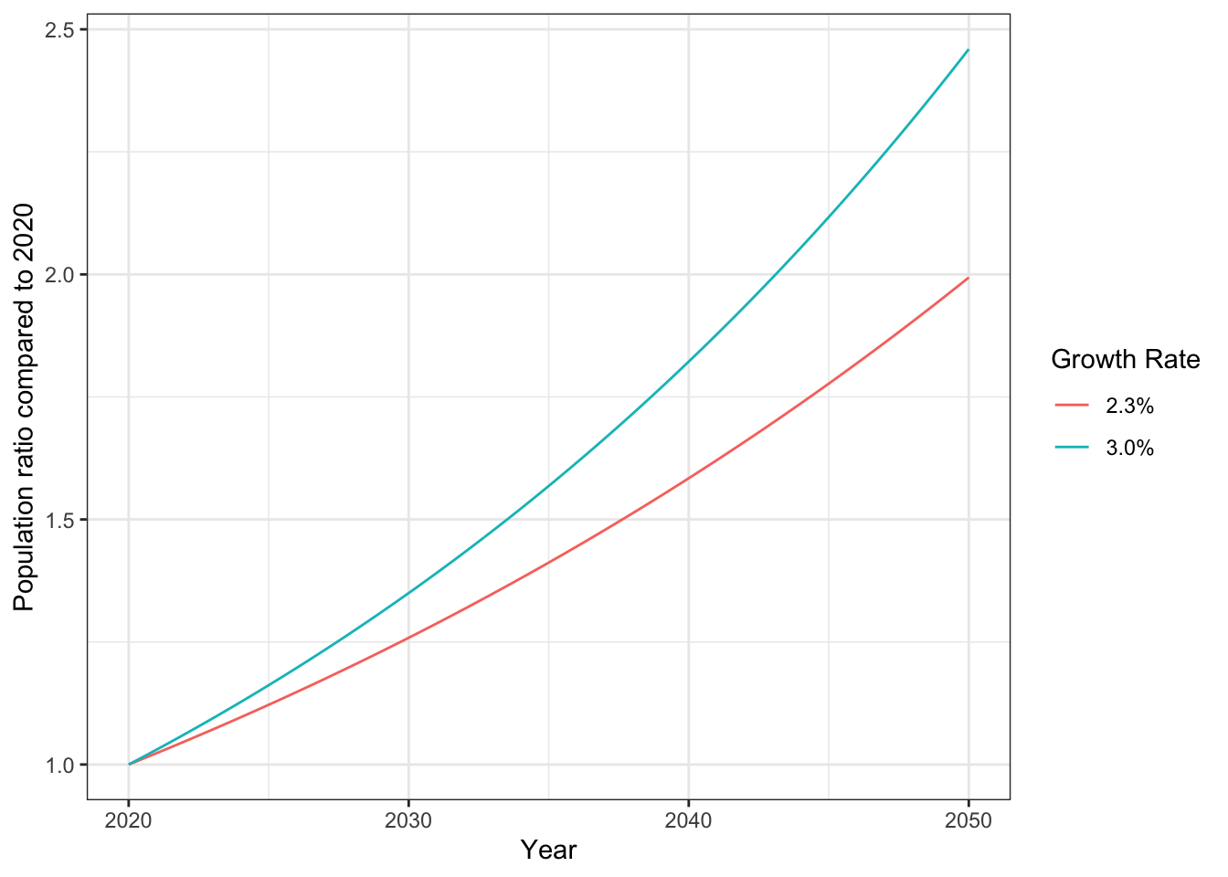
Many human populations and other economic variables grow at a rate of 1% to 3% per year. There are situations that grow at a considerably higher rate, like the populations of microorganisms.

A wastewater treatment plant uses bacteria to convert organic compounds in sewage into methane gas and inert material. This species of bacteria replicates every ten minutes. If you start with one bacterium, how many will you have after twenty-four hours?

In this case the replication rate is 100% per 10 minutes, or 600% percent per hour. So after 24 hours, the population of bacteria is $1*exp^{6*24} = 3.455\times10^62$. We can plot this growth over time, though if we don’t use a logarithmic axis it’s pretty hard to see what is going on.

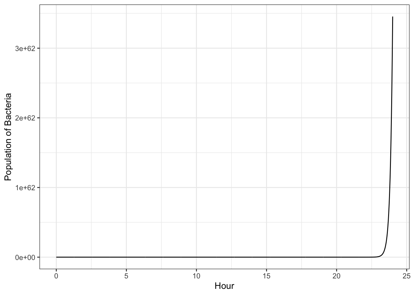
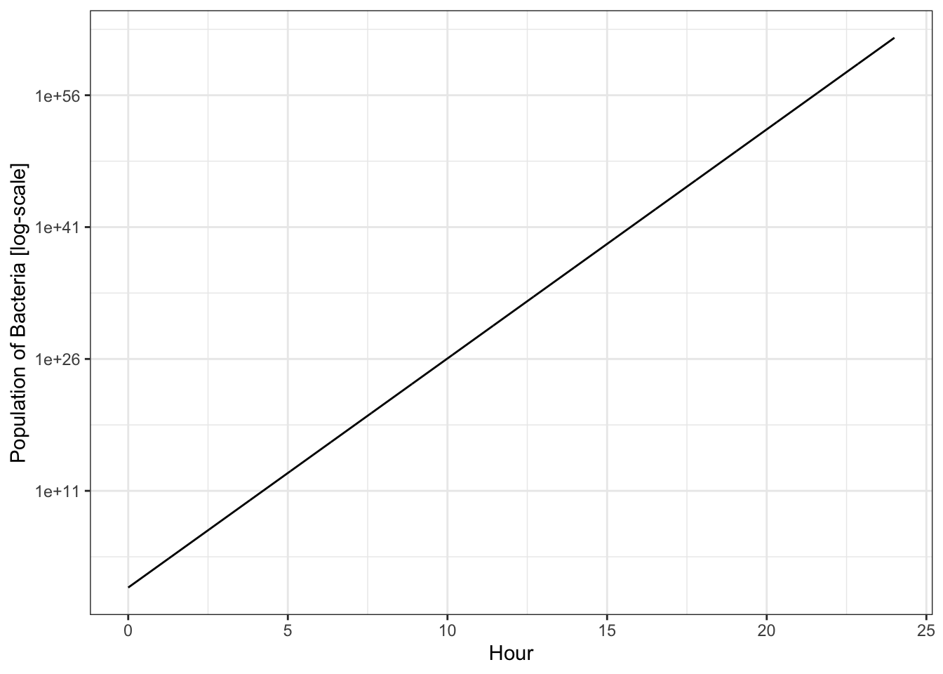
It’s important to point out that limitless exponential growth is almost nonexistent in the real world. Bacteria will only have ideal conditions to grow for a short time before resources become scarce and the population growth rate slows.

Unit Summary

The time value of money means that $100 now is worth more than $100 in the future because of risk, inflation, and opportunity cost. This makes interest a powerful tool in funding projects with things like mortgages, bonds, sinking funds, and toll-based financing. Cash flow diagrams provide an easy way to organize the cash flows of projects over long periods of time. Using equivalence equations for present value, future value, and annuities allows us to calculate the net present value (NPV) from a cash flow diagram, which determines if a project will be profitable. We must pick an appropriate discount rate in order to correctly calculate the present value of future cash flows and to meet our minimum acceptable rate of return (MARR). Exponential growth also has many other applications to civil engineering besides finance, including population growth and traffic predictions.

Ultimately, though, decisions cannot be based on finances alone. They must also incorporate costs and benefits that do not have monetary values, either by determining a value for them or by using a suitable weighting system for different categories. Sustainable infrastructure can only be achieved if all of these factors are considered.

annuity (A): a series of equal payments made over time
bond: financial tool in which an investor loans a sum of money to an organization, and the borrower pays annual interest on the loan until the end date of the bond, at which point they pay back the face value
book value: the initial cost of an asset minus total depreciation
cash flow diagram: a graphical display of cash inflows and outflows over time
Categorical Exclusion (CATEX): a type of federal action known to have no environmental impacts
compounding frequency: the frequency with which the interest on a loan is re-applied to the principal
depreciation: the value of an asset lost over time due to use, found using methods like straight-line or MACRS
discount rate: an interest rate used to determine the present value of a future cash flow
Environmental Assessment (EA): an evaluation of the potential environmental impacts of a proposed federal project
Environmental Impact Study (EIS): an extensive alternatives analysis used to evaluate the environmental impacts of a proposed federal project
Environmental Protection Agency: government agency in charge of determining whether or not a project is safe for the environment
external rate of return (ERR): the discount rate at which the present value of investments is equal to the future value of earnings
factor tables: tool for converting cash flows (PV,FV,A,G) into equivalent time values of money
Finding of NO Significant Impact (FONSI): issued if an environmental assessment finds minimal or negligible impacts
future value (FV): the equivalent future worth of a sum of money or series of payments
gradient (G): a series of equally increasing payments made over time
inflation: the increase in price for goods and services over time
interest: money paid by a borrower to a lender in exchange for the use of their money
internal rate of return (IRR): the discount rate that makes the NPV of a project equal to zero
minimum acceptable rate of return (MARR): the lowest rate of return that a project must earn in order to be worthwhile to an investor
mortgage: a loan to purchase property using that property as collateral, repaid in regular periodic amounts
National Environmental Policy Act (NEPA): a federal law that requires all federal agencies to evaluate the environmental consequences of proposals before making decisions
net present value (NPV): the equivalent present value of all future cash flows
opportunity cost: the potential benefits that are lost when one option is chosen over another
present value (PV): the present worth of a sum of money or series of payments
project assessment: comparing projects using methods such as NPV, ROI, B/C, and incremental B/C
project evaluation matrix: a tool to compare several alternatives across an array of quantitative and qualitative criteria
Record of Decision (ROD): the final decision of the EPA on whether or not a project has acceptable environmental impacts
refinancing: taking out a second loan at a lower interest rate to pay off an original mortgage
return on investment (ROI): the ratio of the equivalent annual earnings to the total investment
risk: the chance that an investment will be less profitable than expected, including the possibility of losing some or all of the original money
sinking funds: a fund where smaller amounts of money are put aside regularly to pay for some larger expense in the future
time value of money: the concept that money now is worth more than the same amount of money later because of risk, inflation, and opportunity cost
toll-based financing: loans to build infrastructure are repaid using future revenue from tolls and service fees
zoning: laws that specify what types of projects can be built in certain areas

Homework

If $2,500 is invested at a rate of 5% compounded annually, what is its future value after 20 years?
You want to deposit a single amount of money now in order to have enough to buy a new car for $25,000 in 10 years. You decide to invest the money in a mutual fund that will earn you 13% interest per year. How much money do you need to deposit now to pay for the car in 10 years?
Marie and Alyssa both decide to put money into a mutual fund where they will accumulate interest at a rate of 7% per year. Marie invests $10,000 when she is 25. Alyssa waits until she is 45 and then invests $35,000.
1. Who will have more money saved by age 65?
2. At what interest rate would they have the same amount of money at age 65?
Consider each cash flow diagram below. Is the financing tool most like a bond, a mortgage, or a sinking fund?

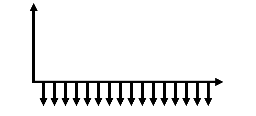
Figure 3.7: A

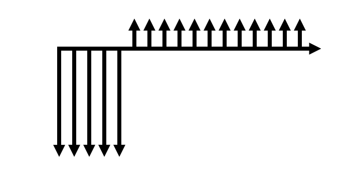
Figure 3.8: B

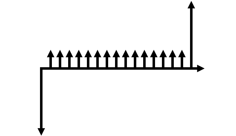
Figure 3.9: C
Draw a cash flow diagram for each of the following scenarios from John’s perspective. Label arrows with cash values.
1. John decides to take out a $300,000 mortgage for a new home. It is repaid in monthly payments of $1,300 over the next 30 years.
2. John buys a boat for $80k (year 0), which he will sell in five years for $40k (year 5). Each year the boat requires $1,000 in maintenance and upkeep, including the year he sells it.
3. John purchases a $1,500 bond (year 0) that will pay 5% interest on its face value for the next 10 years. He will also be repaid the initial $1,500 investment at the end of the 10 year period together with his interest for that year.
4. John creates a retirement savings plan, in which he will invest $10,000 a year for the next 10 years. After that point, he will begin withdrawing $500 a year in perpetuity.
TJ borrows $150,000 from the bank at a rate of 3% interest compounded annually. If he pays back the loan in 20 equal payments over the next 20 years, how much will each payment be? Draw a cash flow diagram as part of your solution.
Ben can buy a bond with a face value of $1000 paying at 6% interest for five more years. What is the present value of this bond if Ben’s personal discount rate is 5%? What is the present value at a 7% discount rate? Note: to solve this problem, first draw the cash flow diagram for the bond. Then, determine the present value of these flows using the different discount rate.
Jared’s parents give him an old car that will last for 10 more years as long as he keeps repairing it. The car needs $200 worth of repairs the first year, and the maintenance costs will increase by $50 each year afterwards. How much money does Jared need to invest now at an 8% interest rate to pay for the next 10 years of maintenance on the car? Draw a cash flow diagram as part of your solution.
Alisa wants to install a new $9,000 air conditioning system. Because it is more energy efficient, the system would save $1400 per year in electricity costs. Assuming a discount rate of 7%, how long will it take for the air conditioning system to pay for itself? Draw a cash flow diagram as part of your solution.
The Deluxe Cookie Company decides to buy a new industrial-size oven for $12,000. After 15 years, the salvage value of the machine will be $3,000. Insurance for the oven costs $900 per year. The oven will also use $1,300 worth of electricity per year and require $250 in maintenance at the end of each year. However, the new oven will also save the company $3,600 per year. Assuming an effective annual interest rate of 8%, what is the equivalent present worth of the new oven? Draw a cash flow diagram as part of your solution.
Rachel loves to make tacos, and wants to start a business running a taco truck. The truck and cooking equipment cost $45,000 initially, and she can sell them 14 years later for a salvage value of $11,000. Annual maintenance on the truck and equipment cost $2,500 for each of the 14 years, but she also expects to make a yearly revenue of $10,000. Rachel’s MARR is 9.5%. Determine the NPV and ROI this project; should Rachel go for it? Show your work, either on calculation paper or by annotating an Excel spreadsheet.
Repeat the previous problem, but consider that Rachel can take out a loan at very favorable terms to buy her equipment: 14 years at 2% interest (repaid as an annuity over the next 14 years). Calculate the new NPV and ROI for this project. Should Rachel go for it now?
Repeat the previous problem (where Rachel uses a loan to pay for her taco truck), but consider that demand for tacos is variable. Instead of a constant $10,000 year revenue, the revenue for years 1 through 14 actually ends up following the values listed below. The final revenue value includes the $11000 salvage price. Calculate the NPV and ROI for the project using the variable revenue stream. Plot / chart the net profit (revenue minus expenditures) in each of the 14 years of Rachel’s taco truck. Describe what could happen in year 6.

Yearly revenues: 7000, 10000, 13000, 18000, 11000, 2000, 8000, 12000, 10000, 13000, 9000, 8000, 7000, 21000
Zach owns a company that can produce 180,000 microwaves yearly. The company’s fixed costs are $1,500,000 per year to run the factory, and the variable cost for each microwave is $25. The microwaves sell for $100 each.
1. How many microwaves does Zach’s company need to sell to break even?
2. Zach is considering investing in a new assembly line system that would reduce the variable cost for each microwave from $25 to $20. The new assembly line would cost $450,000 to build. How many microwaves would Zach need to sell for the new assembly line to be worth the investment?
3. Zach decides to build the new assembly line for $450,000. Assuming that all 180,000 microwaves produced are sold at an even rate over the course of the year, what is the payback period for Zach’s investment in the new assembly line?
A pipeline is installed at a cost of $3,400. The annual interest rate is 10%, and annual maintenance costs are $500. It can be salvaged for $900 at the end of a 15 year service life. The pump costs $1.25 per hour to run, and is in operation 800 hours a year. What is the equivalent uniform annual cost (EUAC) of the pipe? Hint: To find the EUAC, simply convert all values into an equivalent annuity.
A new highway passing over a small stream requires the construction of a culvert. The engineer in charge has three options for the type of culvert to be used. A 24 inch RCP will cost $10,000 and have a 25% chance of overtopping each year. A 2 ft by 4 ft box will cost $20,000 and have a 15% chance of overtopping each year. A twin 2 ft by 4 ft box will cost $26,000 and have a 10% chance of overtopping each year. If the culvert is overtopped, it will cost $10,000 to repair. If the annual interest rate is 8%, determine which option is the most economical for each of the following scenarios.
1. The lifetime of each culvert is 15 years.
2. The lifetime of each culvert is 25 years.
3. The lifetime of each culvert is 50 years.
The present value of costs and benefits for five alternatives (plus a do-nothing alternative) are given in the table below. Assume the project continues forever, and use a discount rate of 8%. Identify the preferred alternative based on:
1. ROI
2. NPV
3. B/C
4. Incremental B/C (provide a plot)
  
  Alternative Benefits Costs
  
  Do Nothing 0 5
  
  A 200 40
  
  B 100 20
  
  C 50 25
  
  D 150 30
  
  E 80 15

Alternative	Benefits	Costs
Do Nothing	0	5
A	200	40
B	100	20
C	50	25
D	150	30
E	80	15

The table below shows an evaluation matrix for alternative transportation projects. Identify the preferred alternative using the scores and weights that are given.

Criteria	Weight	Alternative A	Alternative B	Alternative C
Reduce travel time	7	2	5	2
Improve Level-of-Service	2	5	5	2
Improve flexibility	2	5	5	5
Improve access to jobs	8	2	1	5
Reduce non-auto travel times	3	4	3	5
Compatible with local plans	2	2	3	2
Public acceptability	7	5	2	4
Minimizes socioeconomic, cultural, and environmental impacts	5	5	3	3
Cost-effective	8	1	5	3

Consider the project evaluation matrix from the previous problem. How might you change the criteria or the weights to better reflect a sustainability perspective?
After 14 years running her taco truck, Rachel considers whether to invest in a storefront. She will purchase $50,000 of kitchen equipment with cash, which she expects to salvage for $10,000 after 11 years. Her operating costs will increase to $4000 per year, but her revenues will also increase to $15,000. Rachel’s discount rate is 8%, and business profits are taxed at 25%.
1. Using a straight-line depreciation technique, calculate the NPV and ROI for this proposal. Calculate the total (non-discounted) amount paid in taxes.
2. Using the MACRS depreciation technique, calculate the NPV and ROI for this proposal, as well as the total (non-discounted) amount paid in taxes.
3. Which method should Rachel use?
You have the option to purchase a lot on the edge of downtown Provo for $1 Million, and wish to build an apartment tower, which you believe you can complete in one year. You estimate that construction will cost $2.8 million per story, and that annual revenue will follow a function $A = 0.8 + 0.04 s^2$ where $s$ is the number of stories and $A$ is given in millions of dollars, provided the complex is more than one story tall. You have a discount rate of 9% and are planning for a horizon of ten years after construction.
1. Current zoning codes limit your structure to 3 stories. Calculate the NPV and ROI.
2. If you were going to petition the city for a zoning variance, how many stories would you want to build?
Find the EIS for a recent project that interests you. How many alternatives did the EIS consider? What were the criteria on which the alternatives were evaluated? Do you feel that the EIS is sufficiently comprehensive? A database of EIS documents since 2012 is on the EPA website.
Hunter is an environmental engineer. He has been observing a lake where a certain species of fish is increasing in population at a rate of 7% a year. There is also a species of frog that has been declining in population at a rate of 4% each year. There are currently 276 of the fish and 483 frogs in the lake.
1. How many years will it take for the fish population to grow to 500?
2. What will the frog population be in 5 years?
Your friend comes to you with a business proposition, where you agree to buy energy drinks from a manufacturer and sell them directly to customers. Because he’s brought you into this great opportunity, you will give him a certain percentage of your revenues. If you recruit people to sell for the company, then they will give you a percentage of their revenues. In order for the average revenues to exceed the cost of the energy drinks, you will need to recruit at least five other people to sell energy drinks, who will face the same need to recruit. How many rounds of recruiting people to sell energy drinks can you go through before you exceed the population of earth? Is this a sustainable business model?
A small town in Nevada uses a local aquifer as its water source. There are currently 500 people that live in the town, and each uses about 100 gallons of water per day (this may seem like a lot, but it’s actually the average for people in the US). The aquifer currently contains 500 million gallons of water, and it naturally replenishes at a rate of 20 million gallons per year. The population of the town is growing at a rate of 5% per year.
1. At the current rate of population growth, how long will it take for the aquifer to run out of water?
2. The growing town decides to implement a water conservation program to educate their citizens about the limited water supply. Thanks to their efforts, the average water usage drops from 100 gallons a day to 75 gallons a day per person. With the decreased water usage, how long will it take for the aquifer to run out of water?
Imagine a town where the traffic on the main street is increasing at a rate of 7.3% each year. The flow rate will become unacceptable once the traffic reaches 1500 vehicles an hour in its peak hour. At its current peak hour it has about 700 vehicles. How many years does the town have before it needs to find a solution to the increasing traffic?

References

Martland, Carl Douglas. 2012. Toward More Sustainable Infrastructure. Wiley.

Meyer, Michael D., and Eric J. Miller. 2001. Urban Transportation Planning: A Decision-Oriented Approach. 2nd ed. McGraw-Hill.

There are many more tools than can be listed here, and these descriptions are perhaps dangerously oversimplified. But this gives a decent overview for undergraduate engineers.↩︎
A complete discussion of macroeconomic policy in setting and governing interest rates including the role of central banks is outside the scope of this class and the expertise of your instructor.↩︎
There are also formulas for gradients that grow by less than a uniform amount. We will not cover these in this class↩︎
You can also see this as $F/P = (1 + i)^n$, where the factor you want is isolated by the division.↩︎
Example taken from Martland (2012)↩︎
Example drawn from Meyer and Miller (2001)↩︎