1 Introduction
Transportation is the movement of people and goods. Transportation engineering is therefore concerned with designing systems and facilities that allow people and goods to move efficiently and safely.
These people and goods don’t move simply because they want to. Transportation is a derived demand: people need to go to work or school; people want to go somewhere for leisure or entertainment; goods need to get from where they are grown or manufactured to where people will buy them, etc.. Further, the decisions of which transportation projects get built and where requires engineers to communicate with the public and with their elected decision makers. Successful transportation engineers therefore need to understand both the human systems and the infrastructure systems that comprise transportation.
Transportation engineering is absolutely engineering. In this class you will learn how to:
- specify the angles, length, and radii of roadway curves to ensure motorist safety
- specify the thickness of flexible pavement layers
- determine the hourly capacity of a freeway segment
But transportation engineering is also a social science. In this class you will also learn:
- what factors cause people to drive instead of take transit or walk, and how we can measure or influence these factors
- how transportation infrastructure projects are planned and funded
- who is affected by transportation noise, pollution, and other nuisances
Tip 1.1: Terms and Concepts
Perhaps unlike some of your other engineering classes to this point, this class has relatively more terms and concepts in relationship to methods. Understanding the appropriate terms and concepts is essential to your success in this class (and in your career). Think of it as learning a new language. The best way to become proficient in most languages is to memorize vocabulary and speak your language. Terms written in bold should be memorized. In this chapter, we will introduce most of the background topics to set the stage for the more technical engineering concepts and techniques introduced in future chapters.
Fricker & Whitford (2019) captured the idea of transportation systems engineering encompassing multiple different types of engineering with the metaphor of a three-legged stool. The three “legs” of this stool are as follows:
- The components of the system: The work that goes into engineering the vehicles, facilities, and right-of-way that the transportation system uses. This includes highway curves, traffic signal arms, runway pavements, etc.
- Putting the system in place: The work that goes into planning which facilities to build, and how to obtain necessary funding.
- Issues for viability: Understanding, quantifying, and reducing the costs the transportation system places on society. These costs include sustainability issues related to population growth and traffic congestion, vehicle emissions, and transportation safety among others.
1.1 Transportation Concepts and Challenges
A trip is a journey from an origin where the trip starts to a destination where the trip ends. People can make trips for a variety of purposes or reasons: traveling from home to work, or from home to social or recreational activities, or just from one place to another place. Depending on the purpose of the trip, people may be more or less willing to use particular transportation modes, or pay additional money to save a bit of time.
1.1.1 Mobility and Accessibility
Transportation systems have two goals. They need to provide mobility, or the ability to move large numbers of people and goods through space. They also need to provide accessibility, or the ability for those people and goods to reach locations that matter to them.
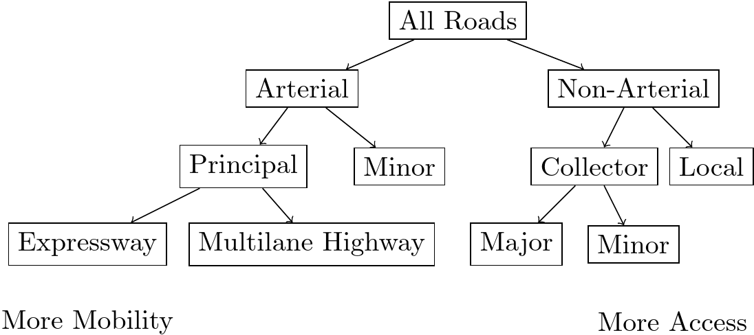
Often, a transportation facility cannot provide both accessibility and mobility effectively at the same time. An expressway (like an interstate freeway) provides great mobility, with large numbers of cars able to move long distances at high speed with very few interruptions. But the things that give a freeway high mobility — space between ramps, uniform traffic flow, no traffic signal control — mean that a freeway has exceptionally poor accessibility. On the other hand, most local roads provide high levels of accessibility but very limited mobility. When people do try to use neighborhood streets for mobility, it causes safety issues, congestion, and other nuisance problems for the people in the neighborhood.
Roads are often grouped into functional classification or functional types that describe their purpose in terms of mobility versus accessibility. Between expressways and local roads are a spectrum of road types providing an array of access / mobility trade-offs. Some of these classes are shown in a chart in Figure 1.1. More information on functional classification is available from Federal Highway Administration (2013).
Building a highway network entirely from roads with one functional classification would not likely result in positive outcomes. Few people want to live or walk beside an expressway or multi-lane highway, and local streets should not be expected to move large volumes of people or goods at high speeds.
Tip 1.2: Functional Classification
Trace your route from your home to the Engineering Building. Can you identify the functional classification for each street or road you use?
1.1.2 Transportation Modes
Of course, roads and road vehicles are not the only way people and goods move around. Different means of moving people and stuff around are called transportation modes. Just as some highway facilities are better for improving mobility or accessibility, different modes excel at different applications.
The most basic mode of transportation — and the primary mode for almost all of history — is walking. It is the only mode available inside of most buildings, and it is how people often transfer between travel modes. Many people continue to walk for transportation even in modern cities, as a form of exercise, to avoid the inconvenience of parking, or for other reasons. Cycling is more modern, but provides many of the same benefits of walking with a bit of added speed at an affordable price. The distance that most people are willing or able to walk or bike can be limited, and many 20th-century cities are not designed in a way that makes doing so pleasant or convenient.
Automobiles provide high mobility and high accessibility, at a price that is high but within the means of many people. Roads and highway bridges for moving vehicles are some of the most common infrastructure facilities that civil engineers of all discipline areas work on, and automobiles are the most common mode in most American cities by an overwhelming margin. On the other hand, the large amount of space and energy consumed per automobile traveler causes serious sustainability issues that will be addressed later.
Aircraft move passengers and goods more quickly than almost any other mode, but at high cost and high energy use. The point-to-point infrastructure required by aircraft is negligible but airports themselves are large, complex pieces of infrastructure requiring careful engineering design.
Rail vehicles can move considerably more people or goods at lower energy expenditures than automobiles, and in some cases at a speed rivaling aircraft. The rail tracks themselves are complex facilities requiring specialized knowledge to design and maintain.
Public transit is an important mode for moving large groups of people in dense areas where automobiles are inefficient, or providing mobility to people who do not drive for a variety of reasons. Transit vehicles may use roads shared with automobiles, dedicated lanes on those roads, or rail systems built above or below ground.
An exhaustive list of all transportation modes is effectively impossible, and new modes (like e-scooters) arise constantly. Other modes that used to be commonplace have become hobbies (like horseback riding) or disappeared entirely (when was the last time you rode in a zeppelin?). Some modes — like oil or natural gas pipelines — can really only be used for one specific purpose. Some trips can only be made by using multiple different modes in succession; places where people transfer between modes (e.g., rail stations or airports) are called intermodal transfer facilities.
Tip 1.3: Intermodal Transfers
Think of the last trip you took to a destination far away from your origin. How many different transportation modes did you use on that trip? How many intermodal transfer facilities did you use?
1.1.3 Transportation Sustainability
The transportation system needs to be sustainable, meaning that the costs of building and operating the system should be able to continue indefinitely. The three dimensions of the “triple bottom line” of sustainability are:
- Economic: the financial resources to run the system must exist perpetually.
- Environmental: the natural resources required to run the system cannot be extracted faster than they are replenished, and the environmental costs must be bearable.
- Social: the benefits of the system should not go to one group while the costs go to a different group.
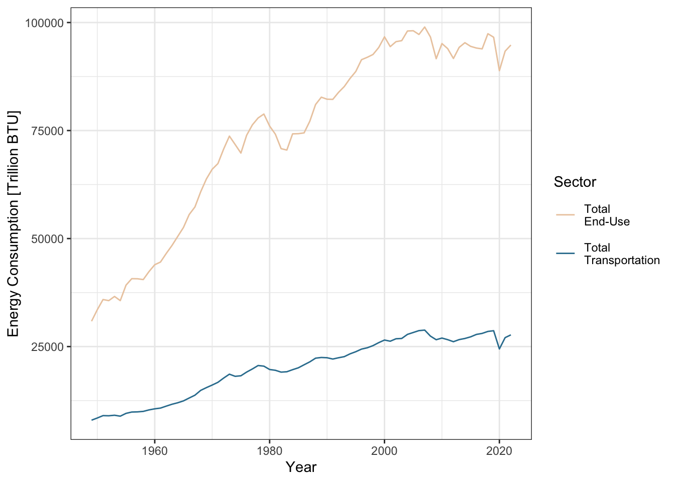
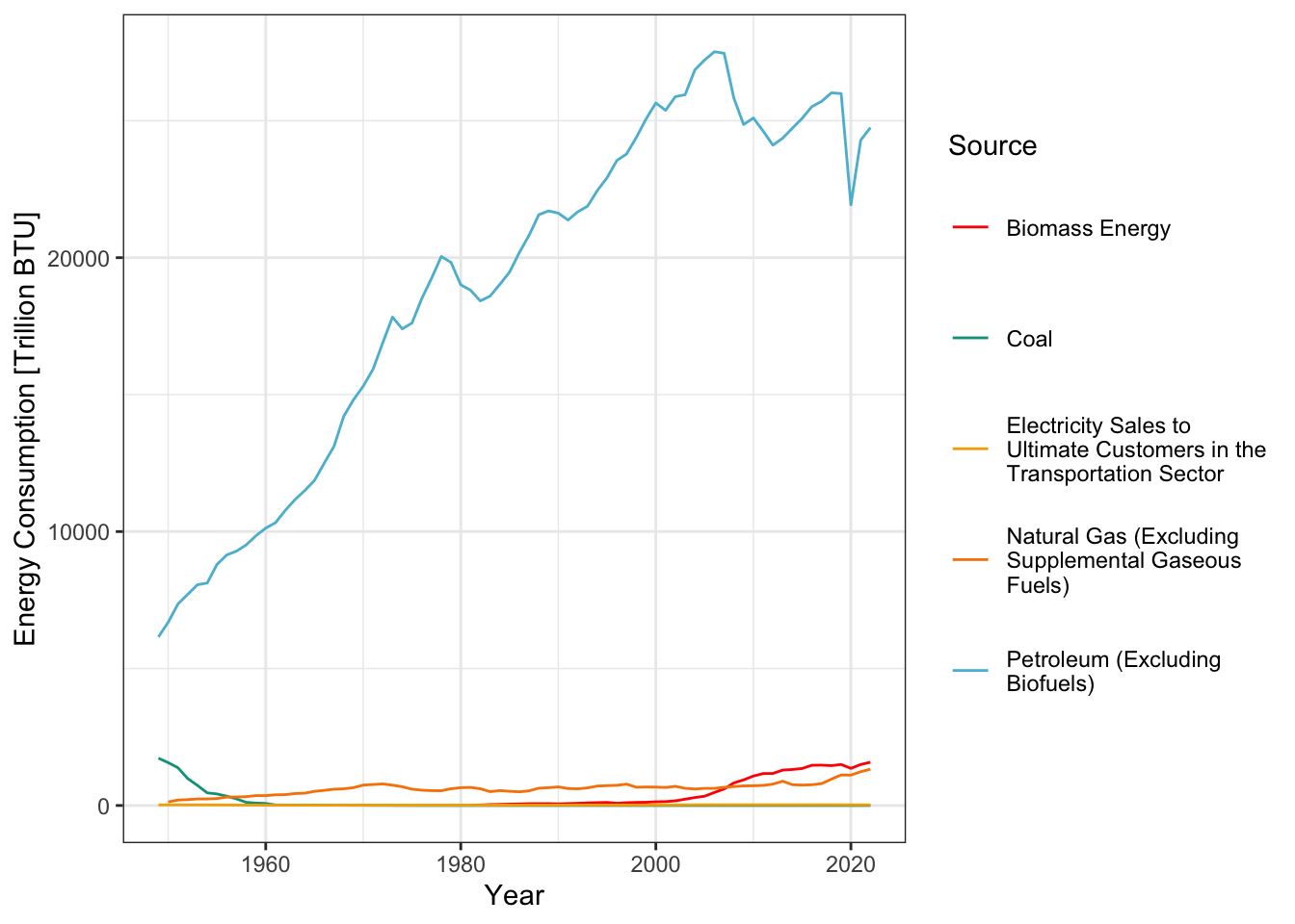
An automobile-dominated transportation system poses many sustainability challenges. Because automobiles are big and heavy, they require a great deal of energy to move. The transportation sector accounts for around 30 percent of all energy use in the United States, and this energy comes overwhelmingly from fossil fuels (see Figure 1.2 and Figure 1.3). Transportation is consequently a major source of air pollution and a primary obstacle to mitigating and adapting to climate change. Further, transportation infrastructure is often built through neighborhoods that do not have the political or economic power to oppose it — or these neighborhoods developed around the transportation infrastructure because the land in those areas was cheaper — meaning that the problems of transportation air pollution and noise are distributed inequitably.
Driving a car is a task that requires skill and attention, but temporary carelessness (often coupled with bad facility design) causes serious safety problems, with well over 40,000 people dying in vehicle crashes in the United States each year. Pedestrians and cyclists are particularly vulnerable.
Facilities for moving and storing cars take up large of amounts of space in cities that could be used for other things, like housing or business. This makes housing and other goods more expensive than they would otherwise be. Additionally, the space required for cars to travel can exceed the growth rate of the population, meaning that a strategy of widening roads to reduce traffic congestion in a growing city is unsustainable.
It is often difficult for certain individuals to use the transportation system. Blind individuals and those with certain other disabilities may not drive, and other people are too young or do not have the financial resources to purchase a car. These people are sometimes considered captive passengers to transit systems. It is also important to ensure that sidewalks, crossings, and transit vehicles are accessible to those who use wheelchairs or require other special accommodations. But the historical practice of engineers minimizing delay for motorists while also minimizing project cost has often led to the needs of these other users being overlooked or ignored. This further contributes to the safety problems addressed earlier.
1.2 The Transportation Planning Process
How does a community decide what transportation infrastructure should be built? Which roads should be widened? Which should be narrowed and converted into community centerpieces? Should there be a transit system, and where should its stations be located? All of these decisions involve many different people, with many different opinions and roles. In the United States and other countries with similar political systems, transportation planning occurs within a democratic process that allows individuals and community groups to have a say in these decisions.
At the end of the day, which transportation infrastructure projects get funded and built are determined by the actions of decision makers. These are officials who are elected or who are appointed by elected representatives: governors, mayors, city councils, state legislators, transportation secretaries, etc.. These people are accountable to the public through elections, and often — especially at more local levels — campaign on which kinds of transportation projects and reforms they support.
A person or group with an interest in the outcome of a transportation decision is a stakeholder. Common stakeholders include:
- Neighborhood and community organizations
- Real estate developers and business organizations
- School districts and universities
- Environmental advocacy groups
- State and local government entities
Often, different groups of stakeholders disagree on which policies will benefit them. Real estate developers may prefer transportation projects that provide maximum access to their properties, and environmental groups may resist projects that harm natural habitats. It is important to have a forum where the voices of these different groups can be heard.
Engineers, planners, economists, and others with technical expertise do not make decisions of what to build. But they are involved in the decision-making process in important ways. Engineers:
- monitor transportation infrastructure performance measures and identify areas of concern
- identify which alternatives could be realistically considered by a community
- evaluate the benefits and costs of these alternatives
- communicate these findings to decision makers and the public
Tip 1.4: UVX
In 2018, a mass rapid transit mode known as Bus Rapid Transit (BRT) began operation in Provo and Orem, branded as UVX. The buses come every 6 minutes during much of the day, and provides good mobility for transit passengers in central Provo and south Orem.
Before 2025, the largest distance between two stops on UVX occurs between the BYU South (by the Engineering Building) and BYU North (by the MTC) stations. The system as originally designed included a stop near the Creamery on Ninth. Some residents of the Tree Streets neighborhood east of campus opposed the project on a number of grounds, citing its expense, the potential for high volumes of bus traffic, and the perceived risk to students at Wasatch Elementary. In an effort to temper some of this opposition, UTA removed the Creamery on Ninth station from the plan. This decision reduced access to the system for residents of Heritage Towers and others in the Tree Streets who might have valued the service.
After Wasatch Elementary moved to a new location, UTA installed a new stop in front of the Music Building. What might you have done differently to please all of these stakeholders?
Federal law since the 1960’s has specified that metropolitan regions create a transportation planning process that is
- Continuing: The planning effort is always going. Every four years, regions create a new 30-year transportation plan. The plans change as preferences and situations change, but planners are always projecting and revising their projections.
- Comprehensive: The transportation plan has to consider more than just transportation projects. It needs to incorporate land use, economic development, and conformity with other federal laws like the Clean Air Act and Title VI of the Civil Rights Act.
- Collaborative: The plan has to be the outcome of a process where all of the various stakeholders have an opportunity to be heard.
This is collectively referred to as the “3C” planning process. Under federal law, every metropolitan region above a certain population size must have a Metropolitan Planning Organization (MPO) which serves as the hub of these planning efforts. The MPO for Utah County is the Mountainland Association of Governments (MAG); the MPO for Salt Lake, Davis, and Weber counties is the Wasatch Front Regional Council (WFRC).
Large transportation projects in the U.S. are heavily funded by the federal government. The process works basically as follows:
- States collect gas tax revenues and send them to the U.S. Treasury.
- Congress specifies through legislation how the money should be distributed back to the states and other priorities.
- The money is distributed to the states through agencies of the U.S. Department of Transportation including the Federal Highway Administration (FHWA), the Federal Transit Administration (FTA), the Federal Rail Administration (FRA), and the Federal Aviation Administration (FAA).
- MPO’s determine which highway and transportation projects are needed, working with various decision makers and stakeholders as described above.
- State departments of transportation and transit agencies build, operate, and maintain transportation infrastructure and services.
Federal laws and oversight processes ensure that a state DOT cannot build a road simply because it wants to; the road has to be identified as a priority by the MPO’s planning process.
1.3 Transportation Demand Forecasting
Transportation is the result of social economic actions: this person needs to go visit someone here, that company needs to ship a product there, etc. This the derived demand idea that we talked about earlier. Further, transportation is an economic equilibrium: the demand for people to go places and do things is constrained by the costs of travel: air fares, tolls, travel time budgets, fuel and energy, etc.
So when engineers are designing and planning transportation systems, we need to apply some basic tools from economics in order to estimate the demand for the transportation systems. Two common tools engineers use are elasticity analysis and travel demand models
WarningNot a physical system
Many systems that you learn about in Civil Engineering are physical systems with known limits and understandable interactions between gravity, forces, and other physical phenomena. In designing a structure, you estimate how much snow and wind will fall on it, and then design the structure to withstand the worst possible snowstorm and the worst possible hurricane and the worst possible earthquake.
The structure will then presumably remain standing through everything.
Transportation demand is an economic system. If you make the price of a good cheap, more people will buy it. If you make roads wider and faster, more people will use them. So simply building the road for the highest conceivable demand isn’t a feasible strategy.
It’s a little like if building stronger buildings created stronger earthquakes.
1.3.1 Elasticity Analysis
When the cost of a good changes, people change how much of that good they buy and use. This is true with transportation as well.
- When transit fares increase, fewer people take transit
- When gasoline prices increase, people buy less gasoline
- When new roads open, more people drive because the cost of driving is lower
The degree to which the amount of a good bought or used changes as a result of a change in its price is called its price elasticity of demand, or simply elasticity. We can represent the price elasticity \(E_d\) of a good as the ratio of the percent change in the quantity consumed (demand) and the percent change in the price,
\[ E_d = \frac{\%\Delta Q}{\% \Delta P} \tag{1.1}\]
This is also sometimes called the shrinkage ratio, because it is the ratio of how much demand shrinks with an increase in price. If we observe the quantity consumed and the price in two periods (\(t\) and \(t+1\)), we can compute the elasticity as
\[\begin{align} E_d & = \frac{\%\Delta Q}{\% \Delta P} \\ & = \frac{(Q_{t + 1} - Q_t) / Q_t}{(P_{t + 1} - P_t) / P_t} \end{align}\] \[ E_d = \frac{P_t(Q_{t + 1} - Q_t)}{Q_t(P_{t + 1} - P_t)} \tag{1.2}\]
Every good has a different elasticity, and different groups of people might be show more elasticity than others. Some goods are elastic, meaning that a percent change in price results in more than a percent change in the quantity consumed (\(E_d < -1\)). Other goods are inelastic meaning that even when the price increases, people still buy almost the same amount (\(-1 < E_d < 0\)). Some goods may behave in more complicated ways. Table 1.1 provides elasticity values for some common transportation goods.
| Good | Price Elasticity |
|---|---|
| Transit Ridership | -0.33 |
| Gasoline | -0.09 |
| Vehicles | -0.89 |
When we know the price elasticity of a good, we can use this information to forecast what may happen when the price changes. We can rearrange Equation 1.2 solving for \(Q_{t+1}\),
\[ Q_{t + 1} = E_d * \frac{Q_t(P_{t + 1} - P_t)}{P_t} + Q_t \tag{1.3}\]
Elasticity is a relatively simplistic measure, and has many limitations. Some of these limitations include:
- Different users will have different price elasticities. Depending on the demographic makeup of your system, you may have higher or lower values. This applies to the trip purposes, times, and modes as well.
- Elasticity for fare hikes and elasticity for fare cuts are usually asymmetrical — you lose more riders when you raise prices than you gain when you lower prices — but many manuals treat them as equivalent.
1.3.2 Travel Demand Modeling
To help identify which roads or transit systems are needed, the MPO will usually operate a computer model of the region. This model, called a travel demand model, has two primary inputs:
The first input is a list of where households and jobs are in a region, including how many households of different incomes and sizes, and jobs of different industry types. To make this list, the region is broken into traffic analysis zones (TAZ): small geographic areas in between major roads that have mostly uniform land uses. Figure 1.4) shows a map of the TAZ system for the WFRC / MAG travel demand model.
The second primary input of the travel model is a transportation network containing road and transit service information. Not every road is represented in a travel model, but rather roads of regional significance. Usually minor arterials and any critical connectors are included, but local roads are left out.
As outputs, the model gives a forecast of traffic congestion and travel times on each road and transit service. Figure 1.5 shows the WFRC / MAG highway network, with links coded based on the PM congestion factor.1
The specific formulation of a travel model is unique to each region, but many models follow a four-step framework.
- Trip Generation: Estimate how many trips are produced from all the households in a TAZ (production), and how many trips are attracted to all the businesses in a TAZ (attraction).
- Trip Distribution: Match the productions and attractions together, getting a start point and an ending point for each trip.
- Mode Choice: Determine how many trips are made on each mode, including transit and carpooling.
- Assignment: Find the shortest path for each trip, accounting for congestion.
When the inputs of the model change — either because the land use changes for a future growth scenario or the transportation networks change because of a new road or rail service — the model predicts what could happen to the transportation network as a result.
The four-step process is also used in smaller-scale transportation planning activities, like planning for traffic generated by a new business or apartment building. Specific details of some of these steps are covered later in this course or in other transportation engineering courses, specifically CE 565, Urban Transportation Planning.
1.3.2.1 ITE Trip Generation
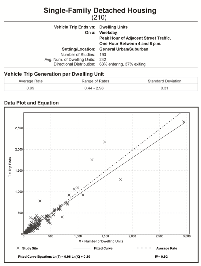
One question that transportation engineers are asked is how much traffic new developments are likely to generate. An important source of trip generation data is the Institute of Transportation Engineering (ITE) Trip Generation Manual. This manual summarizes thousands of data collection activities into equations and rates that can be applied in other contexts. Figure 1.6 shows the Trip Generation Manual information for single family developments in the PM peak by number of dwelling units.
WarningSignificant Digits
Consider the number of significant figures in the previous example. What should you round these estimates to? Given that the precision of the ITE rates is three significant figures, reporting more places than this is mathematically inappropriate. So, \(132.4105\) should be reported as \(132\). If the model had returned \(1,325.89\), then \(1330\) is the mathematically correct response because it has three significant figures, and being more precise than this is misleading about the accuracy of your calculations.
In a practical sense, it may confuse people if you report fractional numbers of vehicles or other indivisible quantities.
1.3.2.2 Mode Choice Analysis
Many problems in transportation require a comparison of discrete options. A person traveling to work might have four alternative modes:
- Drive
- Transit
- Walk
- Bike
Which mode the person chooses will depend on how they value each alternative. Utility is the benefit a person gets from choosing an alternative. If we assume that the person making the choice is rational, then they will choose the alternative that brings them the most utility. But who defines what “rational” is? Presumably every person chooses the alternative that makes sense to them. But as an engineer, how can we see what they are thinking?
The utility \(U\) of an alternative \(i\) has two components: an observable part \(V_i\) that we can measure and an unobservable part \(\varepsilon_i\) that we can’t: \[ U_i = V_i + \varepsilon_i \tag{1.4}\] The observable elements include things like the travel time and the fare. The unobservable parts include things like the person’s individual attitudes and preferences. If the person is choosing from a set of discrete choices \(J\) then they will choose alternative \(i\) if its utility is higher than the utility for all other alternatives. Mathematically we can represent this as an inequality,
\[\begin{align} U_i & > U_j,\; \forall i \neq j \in J\\ V_i + \varepsilon_i &> V_j + \varepsilon_j\\ V_i - V_j &> \varepsilon_j - \varepsilon_i \end{align}\]
This last step suggests that what we really want to know is whether the difference between the parts of utility we can see is bigger than the parts of utility that we can’t.
The observable portion of utility is usually represented with a linear function, \(V_i = X_i \beta_i\). The elements of \(X_i\) are the times and costs that we measure. The coefficients \(\beta\) are estimated from survey data for the population of interest. For example, the equations below are some basic functions estimated from data collected in San Francisco with travel time in minutes and costs in dollars: \[ \begin{aligned} V_{car} & = -0.0514 t_{travel} - 0.49 c_{gas}\\ V_{transit} & = -0.53 -0.0514 t_{travel} - 0.0847 t_{wait} - 0.49 c_{fare}\\ V_{walk} & = -0.207 -0.0514 t_{travel} \\ \end{aligned} \tag{1.5}\] You will learn how to estimate these coefficients and functions in CE 565. For now, you need to know how to calculate observed utility using functions that have been given to you. Be careful with your units!
If we assume that the unobservable piece \(\varepsilon\) has a particular random distribution2 then the probability that alternative \(i\) has the highest utility is
\[ P(i) = \frac{e^{V_i}}{\sum_{j = 1}^J e^{V_j}} \tag{1.6}\]
The probability calculated for one person will tell use which mode that person is most likely to choose. If everyone faces the same choice, then this individual probability is the same as the mode share, or the proportion of people who use each mode. But we can multiply the number of people facing similar choices by the probabilities to get the expected number of people who would choose each mode. The model also gives us a way to forecast what will happen if a service change is made.
Unit Review
Key concepts for this chapter and course:
Succeeding as a transportation engineer requires an understanding of technical, sociological, and political topics.
A transportation system must provide mobility and accessibility, but different facilities and modes are better at providing one or the other.
Automobiles provide good accessibility and mobility, but an automobile-based transportation system faces serious sustainability challenges.
Transportation decisions are made by politicians and appointed officials, with input from engineers and from various stakeholders.
Transportation demand and supply are often understood using elasticity models or a four-step process.
Trip generation rates from the ITE Trip Generation Manual can help engineers determine the total number of trips generated by a development.
Mode choice modeling converts information about people’s preferences into estimated mode shares.
Terms that students should memorize are listed in bold.
Homework
HW 1.1: Transportation Modes
Sort the list of transportation modes given below by increasing accessibility. Then, sort by increasing mobility. Are your two lists perfect inverses of each other? Why or why not?
- Automobile
- Ski lift
- e-Scooter
- Hyperloop
- Passenger Aircraft
- Commuter rail (i.e. FrontRunner)
HW 1.2: Taken For A Ride
Watch the documentary Taken for a Ride. This is available to stream through the Lee Library and Kanopy. Write a short (less than 1 page) reaction to the film. Do you find the argument that there was a concerted effort to dismantle public transportation systems in the United States persuasive? If not, why not? What, if anything, has changed in this area since the film was originally released? What has stayed the same?
HW 1.3: Who Killed The Electric Car?
Watch the documentary Who Killed the Electric Car? This is available for checkout at the Lee Library’s media center, and is also available on some streaming platforms. Write a short (less than 1 page) reaction to the film. Do you find the argument that there was a concerted effort to prevent people from using electric cars persuasive? If not, why? What, if anything, has changed in this area since the film was originally released? What has stayed the same?
HW 1.4: Technologies Research
Choose a transportation technology from the list below. Do a small amount of reading on the technology from internet resources. What is the technology and why did you choose it? Are there any controversies surrounding the technology you chose? What is your opinion on the technology and the impacts it has had (or could have) on society? Cite any and all sources you have used.
- Airbags in passenger cars
- Bluetooth
- Compressed air brake
- Ethanol as an alternative to gasoline
- First bicycle
- Freight Container
- First steam engine
- Global Positioning System (GPS)
- High -speed rail
- Hyperloop
- Magnetic levitation vehicle
- Ride-hailing services
- Seatbelts in private vehicles
- Supersonic transport
HW 1.5: Campus People Mover
The student population at BYU has grown dramatically in recent years. New campus buildings are being built, and more additions to the campus are sure to come. The only places to put these new buildings are where parking lots currently reside on campus. Moving parking to garages at the edges of campus will increase walking distances, but it could help with the safety of pedestrians who have to walk across campus roads. A certain transportation professor suggests that an automated people mover (APM) be considered to help with the movement of students and staff. After some discussion, two conflicting objectives for the APM emerge: First, get students and staff from their vehicles to campus, and back; second, get students to their classes at the various buildings around campus.
How would you describe an Automated People Mover? What are your thoughts on an APM?
Which objective do you think should be adopted? Which one could be more effective?
For the objective you chose in part 2, make a list of at least three stakeholders who should participate in the planning and design of the Campus APM. Why should these stakeholders be consulted? What part do they play in the planning and design of the APM?
HW 1.6: Leg One: Components of the System
For the Automated Campus People Mover (APM) proposed in HW 5, list the necessary components that will make up the system. Why were these components the ones that stood out to you? Do the components change depending on what APM objective is chosen?
HW 1.7: Leg Two: Putting the System in Place
For the Automated Campus People Mover (APM) proposed in HW 5, describe the data to determine if the proposed project will meet the stated needs. Explain your answer and how it will fulfill its purpose.
HW 1.8: Leg Three: Issues for Viability
Discuss the viability issues associated with the Automated Campus People Mover (APM) proposed in HW 5. What could dissuade people from supporting this project? Are there any social issues that could affect the execution of the project?
HW 1.9: Transportation Sustainability Matrix
Build a matrix as shown below, with the 3 elements of sustainability as the rows (Economic, Environmental, and Social sustainability) and the 3 elements of transportation engineering (Components, design / construction, and issues for viability) as the columns. In each cell of the matrix, briefly identify a technology, practice, or policy that you think could help the transportation system in the United States be more sustainable.
| Dimensions of Sustainability | Components | Design / Construction | Issues for Viability |
|---|---|---|---|
| Economic | |||
| Environmental | |||
| Social |
HW 1.10: Land Use and Transportation
Write a short response to the following prompts:
Reflect on how you picked where you live now. How important is the actual dwelling, and how important are the neighborhood’s amenities? How important was the neighborhood’s access to the places you need to get to, or the transportation modes you want to use?
Repeat the previous question, but instead imagine the ideal neighborhood you might want to live in long-term, say in your 40’s. Is the neighborhood you want to live in common or uncommon? Why?
HW 1.11: MPOs
Planning functions in urban areas are carried out by Metropolitan Planning Organizations (MPOs). Answer the following questions for Provo, UT.
What is the MPO’s official name?
How are the cities and counties within its jurisdiction represented on the MPO’s governing body?
What is the current horizon year for the MPO’s long-range transportation plan?
Does the MPO have responsibility for anything besides transportation planning and land use in its jurisdiction?
HW 1.12: Induced Demand
A famous study by Duranton & Turner (2011) found an elasticity of 1.04 for the relationship between the number of roadway kilometers in a metropolitan region and the number of vehicle kilometers travelled in that region. This study controlled carefully for population growth, migration, and other explanatory factors.
UDOT estimated 8,830,000,000 vehicle kilometers travelled in Utah County in 2024. Utah County currently has 4,658 roadway lane-kilometers, and the most recent long range plan proposed adding 1,595 lane-kilometers of new and expanded roads in an effort to reduce traffic congestion.
If the Duranton & Turner (2011) study is correct, what will be the new vehicle kilometers travelled in Utah County after the proposed road expansion? What will be the change in traffic density (vehicles per road lane)? Would there be a change in the number of vehicles per lane on average?
HW 1.13: Transit Elasticity
Two years ago, a local bus system carried 5,964 cash-paying riders when the cash fare was \$0.5 After the system raised the fare to \$0.75 for this year, the ridership dropped to 4,711 riders.
- Calculate the shrinkage ratio for these riders.
- Is the transit demand elastic or inelastic with respect to fare?
- If the agency were to return to a $0.5 fare, how many riders would ride next year?
HW 1.14: ITE Trip Generation
| Independent variable | Number of vehicle trips |
|---|---|
| Acres of Land | 47900 |
| Employees | 4820 |
| Gross Floor Area | 9170 |
The ITE Trip Generation manual was used to get 3 separate estimates of vehicle trip ends per weekday that would be produced by a new drinking water treatment plant near Provo, UT. The results are shown in the table above. A colleague in your firm says, “Always use the highest value. If you do that, then you can always account for the highest number of vehicles and you will have a conservative roadway design.” What might be a good argument against such a philosophy, and what might be the negative consequences of following your colleague’s recommendation?
HW 1.15: ITE Trip Rates
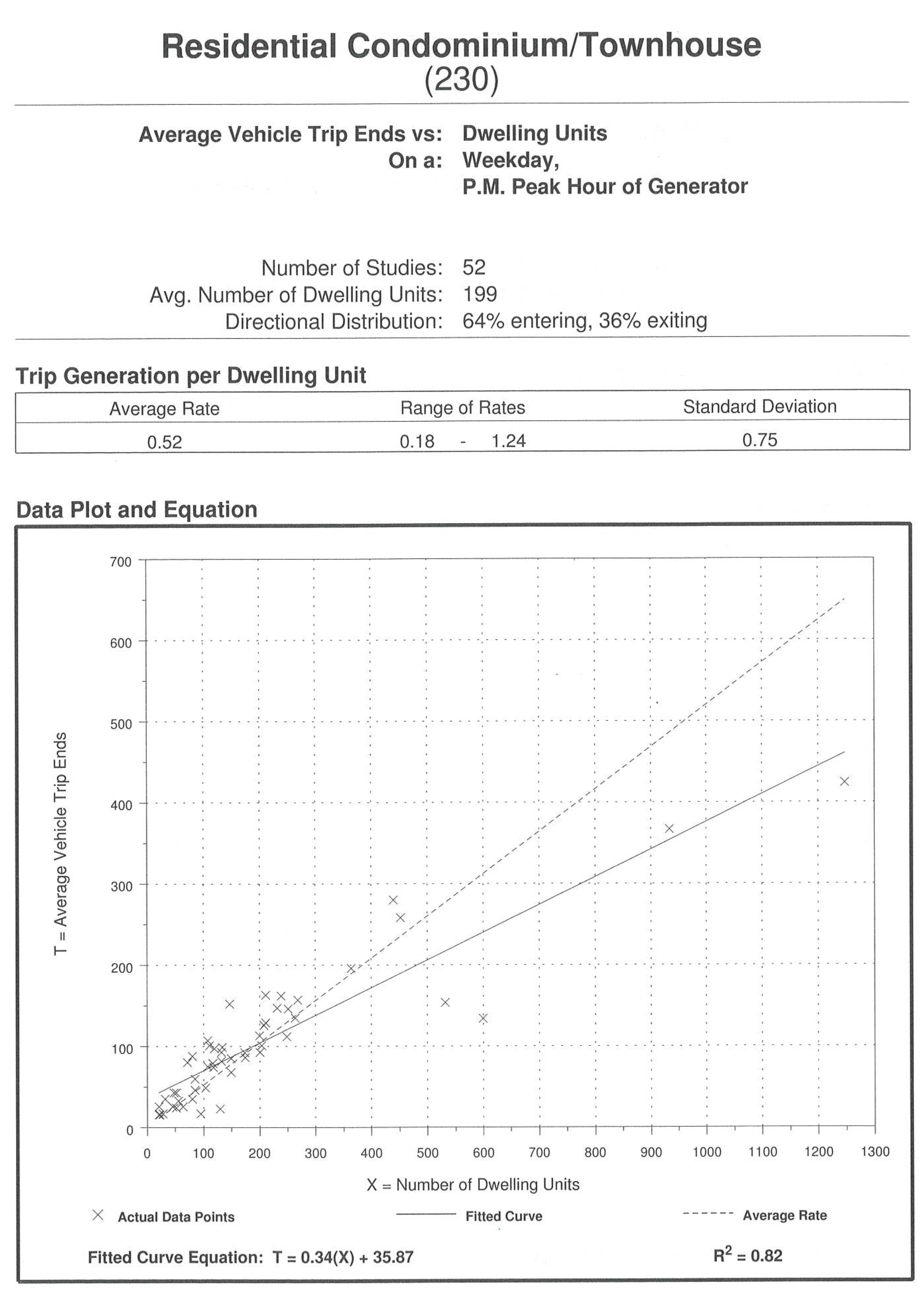
You are advising a developer constructing 75 residential townhomes, and you are worried about trips entering the site at an access road during the PM peak period. The figure above gives the ITE Trip Generation data report for this land use.
If you use the average rate, how many trips should you use in your design?
If you use the fitted curve, how many trips should you use in your design?
HW 1.16: Airport Stakeholders
There are a number of pilots who fly small aircraft into the Heber airport regularly. However, the 1100-foot airstrip limits the number and kind of aircraft that can safely land and takeoff at Heber. There is an air taxi company that would like to fly regular daily service from Heber to Salt Lake in a 12-passenger aircraft that requires a 2500-foot runway. Doing this would mean a whole new airport. There is a vacant lot about 3 miles from the existing airport that could fulfill the necessary requirements if the air-taxi service. The proposed airport relocation would involve building a runway across some land that could be developed for other purposes including residential, educational, and recreational activities. Develop a list of three stakeholders most likely to be in favor of the new airport and a list of three stakeholders most likely to be opposed. Indicate for each stakeholder their main argument(s) for their position.
HW 1.17: Mode Choice In Transportation
A consultant3 is using the mode choice model utility equation \[ V_m = B_m - 0.05\mathrm(time)_m - 0.25\mathrm(cost)_m \]
to predict mode shares between two zones. Auto (\(B_{auto} = 2.1\)) takes 16 minutes and gas costs $2.50; carpool (\(B_{carpool} = 1.2\)) takes 21 minutes but the gas cost per passenger is only $0.80; transit (\(B_{transit} = 0\)) takes 30 minutes and the fare is $0.75.
- Calculate the mode choice utilities and mode shares for this situation.
- To incentivize alternative modes, the businesses at the destination end have determined to add a parking fee of $3 for automobiles that aren’t a part of carpools, and pay for the transit passes for employees. What will be the new mode choice utilities and mode shares predicted by this model?
HW 1.18: Elements Of Mode Choice
For each of the following elements that might affect a person’s mode choice, classify whether each element would likely be observable or unobservable to an engineer studying mode choices. How might each element affect the person’s mode choice?
- The local transit fare
- A person’s claustrophobia
- The number of cars a person owns
- The local gasoline price
- The city a person went to college in
- How many transfers it would take to get from a person’s home to their work on the bus.
HW 1.19: Utility Equation Reasoning
In the utility equations shown in Equation 1.5, most of the coefficients are negative. Why is this? What does this have to do with transportation being a derived demand?
HW 1.20: Coefficient Reasoning
Compare the utility coefficients for travel time and waiting time for transit in Equation 1.5. What does this say about how people feel about waiting for transit?
HW 1.21: Personal Utility
| Mode | Constant | Travel Time | Wait Time |
|---|---|---|---|
| Car | 0.0000 | -0.0354 | 0.0000 |
| Transit | -0.7390 | -0.0354 | -0.0512 |
| Bike | -1.1890 | -0.0354 | 0.0000 |
| Walk | -0.3775 | -0.0354 | 0.0000 |
The utility coefficients for a four-mode system are given in the table above. Construct the mode choice utility equations using these coefficients, and then answer the following parts:
- Compute Dr. Macfarlane’s mode choice probabilities. Dr. Macfarlane has the following travel times from his home to the Engineering Building:
- Bus; 29 minutes travel time with a 10 minute wait
- Car; 12 minutes
- Walk; 55 minutes
- Bike; 19 minutes
- Compute your own mode choice probabilities. Use Google Maps or an equivalent tool to find how long your trip from your home to the Engineering Building would be by bus, car, walk, and bike. Assume you can park at the EB.
- On your last trip to campus did you choose the alternative with the highest utility? Why or why not? If not, is your reason something that could be “observed” in a utility model?
References
Duranton, G., & Turner, M. A. (2011). The Fundamental Law of Road Congestion: Evidence from US Cities. American Economic Review, 101(6), 2616–2652. https://doi.org/10.1257/aer.101.6.2616
Federal Highway Administration. (2013). Highway functional classification concepts, criteria and procedures. https://www.fhwa.dot.gov/planning/processes/statewide/related/highway_functional_classifications/.
Fricker, J. D., & Whitford, R. K. (2019). Fundamentals of transportation engineering (2nd ed.). AcademicPub.
Train, K. E. (2009). Discrete choice methods with simulation. Cambridge university press.