| Vehicle | Time [s] | Headway [s] |
|---|---|---|
| 1 | 0.00 | NA |
| 2 | 17.87 | 17.87 |
| 3 | 33.10 | 15.23 |
| 4 | 39.94 | 6.84 |
| 5 | 43.56 | 3.62 |
| 6 | 49.91 | 6.35 |
| 7 | 53.28 | 3.37 |
| 8 | 57.06 | 3.78 |
| 9 | 61.74 | 4.68 |
| 10 | 66.25 | 4.51 |
2 Traffic Streams
In order to design effective roads, it is important for engineers to be able to describe traffic flow and operation characteristics on those facilities. In this unit, you will learn how to:
- Conduct activities to measure traffic stream characteristics (volume, speed, and density) and analyze field data to estimate values for traffic stream parameters, including hypothesis tests.
- Analyze a standard traffic flow model (i.e., Greenshields Model) for observed traffic data and understand the randomness of traffic flow characteristics.
- Understand the concept of level of service (LOS) and capacity and evaluate the performance of basic roadway segments using standard procedures based on this concept.
2.1 Traffic Characteristics
2.1.1 Headway and Flow Rate
The most elementary traffic stream characteristic is the headway, or the time that elapses between the same point on two consecutive vehicles. If we were to watch a video of 10 vehicles and time when the front axle of each vehicle drove over a line on the roadway, we might end up with data that looks like Table 2.1. The headway \(h\) is simply the difference in the timestamps between consecutive vehicles, and has the units of “time per vehicle.” Note that the first headway is unknown, because we didn’t observe the time that Vehicle 0 passed our observation point.
The average headway \(\bar{h}\) is simply the average of all the headway measurements in a period, and for the example in Table 2.1 is \[\begin{align*}
\bar{h} &= \frac{17.9 + 15.2 + \ldots + 4.51 } {9}\\
&= 7.36 \mathrm{\ seconds\ per \ vehicle}
\end{align*}\]
The inverse of the average headway has an important interpretation, which is the flow rate — denoted with the variable \(q\) and with units of vehicles per time — of the road: \[
q = \frac{1}{\bar{h}}
\tag{2.1}\] In our example, the flow rate is \(1 / 7.36 = 0.136\) vehicles per second. Engineers will usually present flow rates in the more intuitive units of vehicles per hour, which for our example is 489 vehicles per hour.
2.1.2 Volume
A closely related measure to flow rate is the volume of the road, which we will denote with a capital \(V\). The volume is the count of vehicles that pass a point on a road within a specific time frame. The most common volumes used in highway analysis are daily volumes, hourly volumes, and 15-minute volumes. Volume data can be collected by permanent automatic counters that use magnets or radar, by temporary automatic counters that use pneumatic tubes stretched across the road, or by using workers to watch sites or a video feed.
If the flow rate \(q\) is constant for an hour, then \(V=q\) for that hour. But flow rates are variable within hours, within days, and for different days of the week and year.
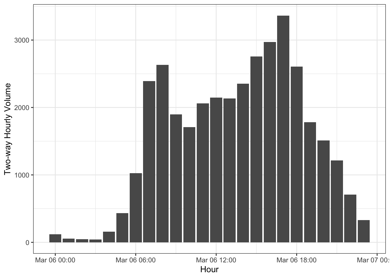
Figure 2.1 shows the two-way hourly volumes measured on Tuesday March 6, 2018 at UDOT’s permanent count station on North University Avenue near the Riverwoods in Provo. As you can see, there is a morning peak around 8 AM as people travel to work and school. There is also a PM peak around 6 PM, as people driving home from work travel alongside people going to evening activities. This is a fairly typical pattern for many urban streets.
The amount of peaking within the peak hour is an important design element; the Peak Hour Factor (PHF) is the ratio of the peak hour volume to the peak 15-minute volume were it to continue for an hour: \[ PHF = \frac{V}{4*V_{15}} \tag{2.2}\]
If all of a road’s peak hour volume occurs in only one 15-minute period, the PHF will be 0.25, and if a road has constant volume for the entire peak hour, then PHF will 1.
Figure 2.2 shows the two-way daily volumes at the same count station measured every day in 2018. In this plot, we break out weekdays, Saturdays, and Sundays / holidays from each other because traffic patterns are so different on those days. There is also seasonal variation, with slightly higher traffic during the school year and lower traffic during the December holidays.
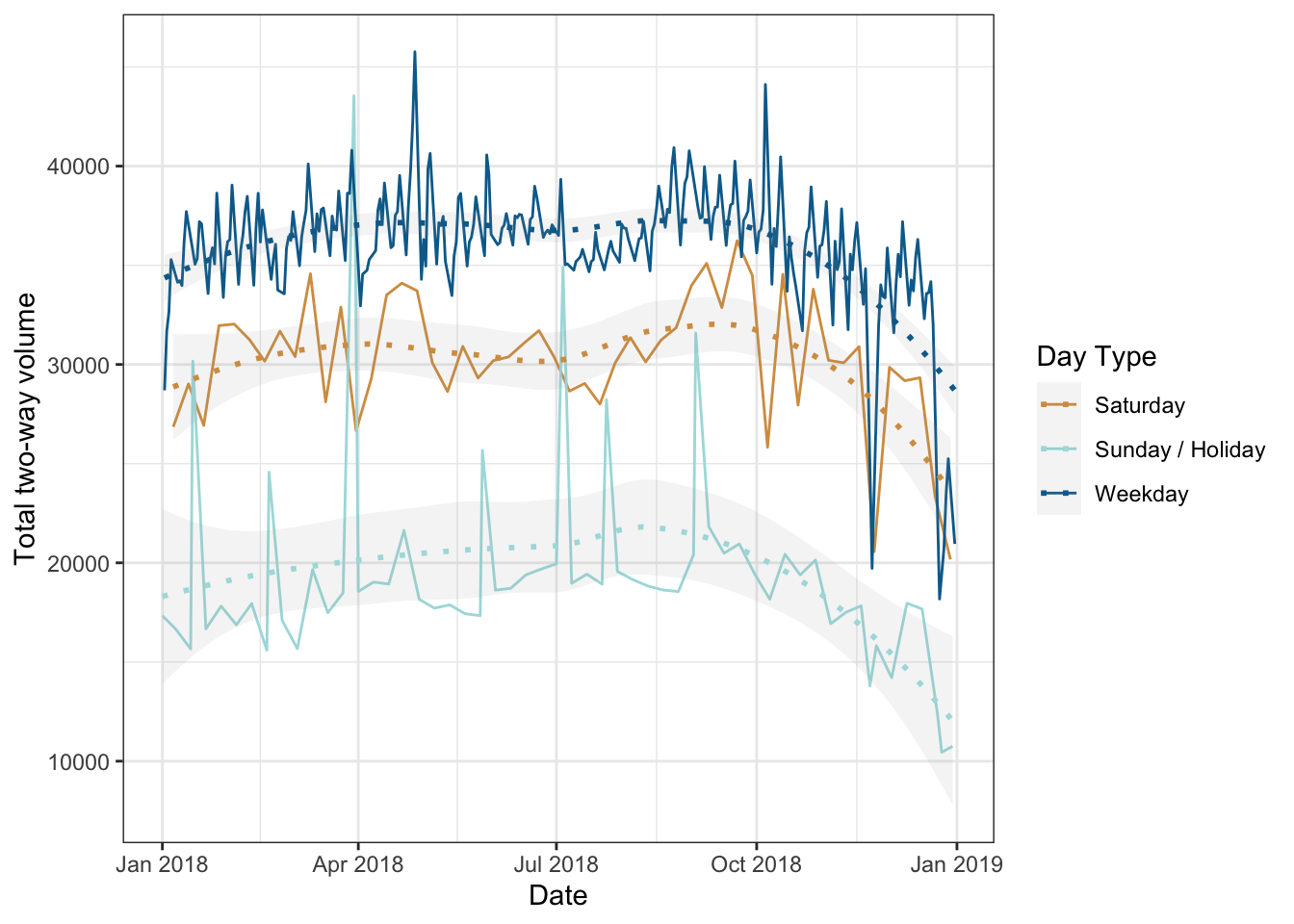
The Average Annual Daily Traffic (AADT) is the average of all the two-way traffic on a road for all days of the year. For the count data in Figure 2.2, this value is 32,391. AADT is an important design consideration. In many design applications, we want to remove weekend and holiday traffic because they are so different, leaving us with Average Annual WeekDay Traffic (AAWDT). For the count data in Figure 2.2 this value is 36,035; AAWDT will usually be a little bit higher than AADT.
The ratio of peak hour volume on a typical day to AADT on a road is a value called its \(K\) factor, \[ K = \frac{V_{peak}}{AADT} \tag{2.3}\] Most roads usually have a \(K\) factor around \(0.1\). A “typical” day is usually understood to mean a weekday without unusual weather or demand conditions, so a Tuesday, Wednesday, or Thursday during the school year is sufficient.
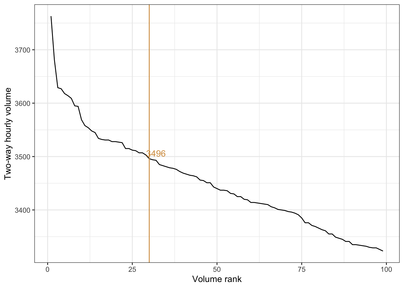
It is irresponsible to build a road for its maximum expected volume; this would mean lots of overbuilding and wasted resources. One standard is to take the 30th highest hourly volume as the design hourly volume. Figure 2.3 arranges all the hourly volumes from the counting station from highest to lowest. The 30th highest volume is 3,496 vehicles per hour.
2.1.2.1 Volumes on roads without counters
Most roads do not have permanent counting stations, meaning that computing design hourly volumes and AADT for a given road is not as trivial as in the previous examples. Instead, engineers reference permanent counting stations to develop seasonal adjustment factors. These factors can then be used to scale hourly counts to obtain design volumes.
2.1.3 Speeds
Vehicle speed is defined as the distance a vehicle travels in a particular amount of time. The two most common units of speed, which we denote as \(v\), are miles per hour (mph, more familiar to motorists) and feet per second (fps, useful when designing road facilities measured in feet). There are two different definitions of measuring mean vehicle speed:
- Time mean speed: using radar or some other technology to measure the speed of vehicles passing a particular point on the road over the course of a time period.
- Space mean speed: using paired tubes or cameras to measure how long it takes a vehicle to travel a particular measured distance on a corridor. Or, equivalently, measure the average speed of multiple vehicles along a corridor at a single instant of time.
If we use method 1 (spot speeds) we can calculate the time mean speed \[ \bar{v}_{time}= \frac{1}{N}\sum^{N}_{i = 1} v_i \tag{2.4}\] where \(N\) is the total number of vehicles measured. This is a simple average of the measured speeds.
Method 2 results in a different definition of the average speed, called the space mean speed. The space mean speed can also be derived as the harmonic mean of the spot speeds, \[ \bar{v}_{space} = \frac{N}{\sum^{N}_{i = 1} 1 / v_i} \tag{2.5}\] The time mean speed will always be a little bit higher than the space mean speed, because vehicles do not drive exactly the same speed through a corridor.
| Vehicle | Time [s] | Speed [fps] |
|---|---|---|
| 1 | 6.69 | 44.9 |
| 2 | 5.72 | 52.5 |
| 3 | 6.18 | 48.5 |
| 4 | 6.32 | 47.5 |
| 5 | 6.20 | 48.4 |
| 6 | 5.95 | 50.4 |
| 7 | 6.76 | 44.4 |
| 8 | 5.95 | 50.4 |
| 9 | 7.01 | 42.8 |
| 10 | 5.97 | 50.3 |
The speed at which vehicles travel — as expected in design and in actuality — is a critical design parameter for a road. Highways with more of a mobility role will have higher design speeds, with longer, gentler curves and fewer obstacles. Local streets with a more accessibility role should not be designed in a way that people feel safe traveling on them at high speeds.
Regardless of how the road is designed, the road should have a speed limit that indicates to motorists what a safe speed is for that road. Current design standards encoded in the Manual on Uniform Traffic Control Devices (MUTCD, see Section 3.2) suggest that the speed limit should be set at the \(85^{th}\) percentile speed of vehicles observed on the roadway. This recognizes the fact that some people will drive faster than the speed limit, but also that having a speed limit that most people do not observe undermines the purpose of speed limits.
Tip 2.1: Is this the best way to set a speed limit?
Many have criticized the \(85^{th}\) percentile speed standard, saying that it results in perpetually increasing speeds. If 85% of people drive 35 mph on a road with a 25 mph speed limit, current engineering practice would suggest raising the speed limit to 35 mph. But would many motorists then start driving 40 mph, knowing that they are unlikely to be ticketed for a minor speed infraction?
Is there something engineers should do to address high speeds on a road besides raising the speed limit?
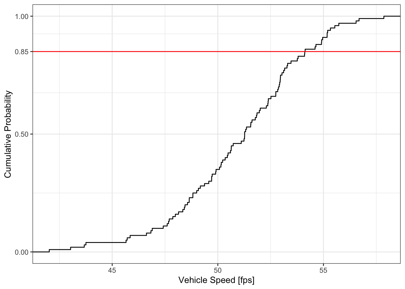
Figure 2.4 shows a set of 100 measured vehicle speeds on a particular roadway, arranged into a cumulative probability curve. The time mean speed of these vehicles is 51 fps, effectively equal to the \(50^{th}\) percentile (or median) speed. But the \(85^{th}\) percentile speed is a bit higher, at 54.1 fps.
Recall from basic statistics that as the number observations in a sample increases, the margin of error between an an estimate of the sample mean and the true population mean decreases. An issue that engineers have to consider is whether they are able to have confidence that their estimate of the \(85^{th}\) percentile speed is within a particular margin of error. The number of observations required to estimate a percentile within a given margin of error at a particular confidence level is \[ N = \frac{\sigma^2 z^2(2 + U^2)}{2 E^2} \tag{2.6}\] where \(\sigma\) is the sample standard deviation, \(z\) is the number of standard deviations from the mean associated with a particular two-sided confidence interval (see Table 2.3), and \(E\) is the desired margin of error (in the same units as \(\sigma\)). The centrality adjustment \(U = 0\) if estimating the mean or median, and \(U = 1.04\) if estimating the \(85^{th}\) percentile (more observations are necessary to confidently estimate numbers farther from the median of the distribution).
| Confidence Level | $z$-score |
|---|---|
| 0.80 | 1.281552 |
| 0.90 | 1.644854 |
| 0.95 | 1.959964 |
| 0.99 | 2.575829 |
2.1.4 Density and Occupancy
Besides volume and speed, the third fundamental traffic flow characteristic is the traffic density. Density will be represented as \(k\) \[ k = \frac{V}{lN} \tag{2.7}\] where \(l\) is the length of the road (usually in miles), and \(N\) is the number of lanes on the road. This means that the units of density are often given as vehicles per mile per lane. Even though density is the last of the three fundamental characteristics we have introduced, in many ways it is the most obvious characteristic; you can look out at any road and immediately see whether the road is empty, jammed, or something in between.
Note 2.6: I-15 Density
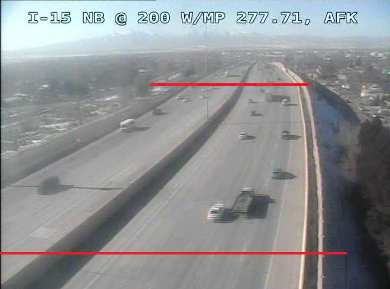
The red lines on the traffic camera image above are 540 feet apart. Calculate the density in vehicles per mile per lane for each side of the freeway, ignoring the carpool / HOV lane.
I can count 9 vehicles in the southbound lanes, and 10 vehicles in the northbound lanes. There are five general-purpose lanes in each direction. This makes the density
\[\begin{align*} k_{nb}&= \frac{V}{lN}\\ &= \frac{10}{540 / 5280 * 5} \\ &= 19.6 \quad \mathrm{vehicles \ per \ mile \ per \ lane}\\ k_{sb}&= \frac{9}{540 / 5280 * 5} \\ &= 17.6 \quad \mathrm{vehicles \ per \ mile \ per \ lane} \end{align*}\]
With flow rate in vehicles per time, speed in distance per time, and density in vehicles per distance, it is possible to construct the fundamental equation of traffic flow, \[ q = kv \tag{2.8}\] We will explore this fundamental relationship more in Section 2.2. For now, note that in order for there to be a high flow of vehicles, the density of traffic and the average traffic speed must be high. Unfortunately, traffic often slows down when the density of traffic increases, meaning that traffic flow is an optimization problem between these two variables.
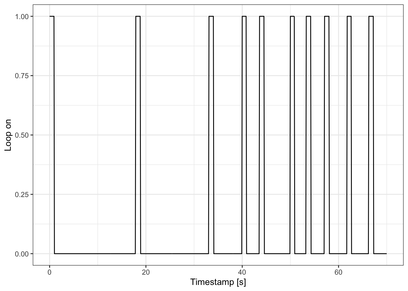
Besides being the most obvious characteristic, density is also usually among the most readily available measures to traffic engineers, along with volume. Permanent magnetic loop detectors installed in the road measure whenever a large metal object is present on top of them. The data from such detectors generates a signal that flips between two binary states: off / 0 when there is not a vehicle above the detector and on / 1 when there is a vehicle. Figure 2.5 illustrates what this might look like for the headway data shown in Table 2.1.
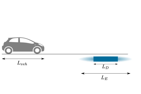
The amount of time that the detector records a vehicle as present \(t(P)\) depends on three elements: how long the vehicle is \(L_V\), how fast the vehicle is traveling \(v\), and the “effective length” of the detector \(L_E\). \[ t(P) = \frac{L_{veh} + L_E}{v} \tag{2.9}\] The effective length is not the same thing as the actual length of the detector \(L_D\), because magnetic loops can be activated before the vehicle is actually over the detector. The different lengths at play are illustrated in Figure 2.6.
The data from loop detectors immediately gives two traffic characteristics:
- The number of times the detector is activated is a count of the volume and be easily converted into a flow rate \(q\)
- The percent of time the detector is activated is the same as the percent of roadway space occupied by vehicles, a measure called occupancy, \(O\).
Occupancy and density are directly related to each other by the length of vehicles in the traffic stream, \[ k = \frac{O}{L_{veh}} \tag{2.10}\] Of course, the correct density must be based on the actual occupancy of the road \(O_{act}\), and not on the apparent occupancy \(O_{app}\) measured from detectors with inflated effective lengths. But \(O_{app}\) can be converted to \(O_{act}\) using a ratio of these lengths, \[ O_{act} = O_{app}\frac{L_{veh}}{L_{veh} + L_E} \tag{2.11}\]
2.2 Macroscopic Traffic Flow
Everyone has driven on an empty road, in the middle of the night or on a Sunday morning when vehicle density on the road is almost zero and you can drive at whatever speed you feel is appropriate. Everyone has also driven on a road in a total traffic jam, when traffic stops completely because the density of cars on the road far exceeds the capacity of the road. Most of the time, roads operate somewhere between these two extremes. It might be useful to build a mathematical model that can describe how speed and density relate to each other.
A simple model known as the Greenshields model (1934) makes velocity \(v\) a function of the density \(k\). The model is a simple line from the free-flow speed \(v_f\) that cars drive when the road is empty and density \(k\) is \(0\), to the jam density \(k_j\) that keeps cars from moving at all and speed \(v\) is \(0\).
\[ v = v_f(1 - k/k_j) \tag{2.12}\]
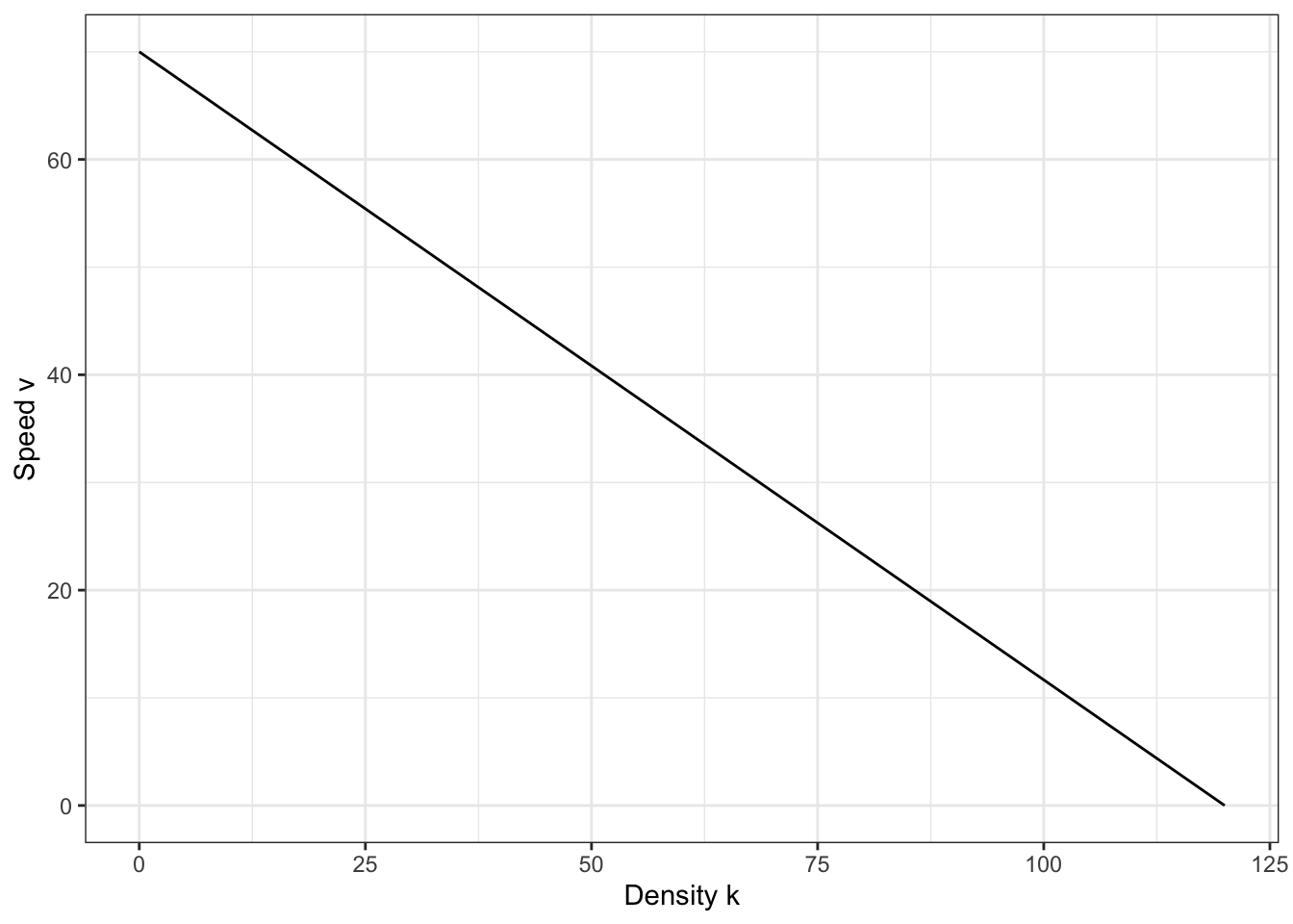
Figure Figure 2.7 shows this simple speed-density model for a road where the free flow speed \(v_f\) is 70 miles per hour and the jam density is 120 vehicles per mile per lane.
The Greenshields model is a very simple model and doesn’t represent traffic perfectly, but there are many things we can observe about traffic from looking at this model. We know from Equation 2.8 that flow is a function of the speed and density and \(v = q / k\). We can use this identity to derive a mathematical model for the flow as a function of the density.
\[\begin{align} v &= v_f(1 - k/k_j) \\ q / k &= v_f(1 - k/k_j)\\ \end{align}\] \[ q = v_f k - v_f k^2/k_j \tag{2.13}\]
This model is a parabola, which is illustrated in Figure 2.8. When the density on a road is zero, the flow is zero because there are no vehicles to count. And when there is a complete traffic jam, the flow is also zero because the velocity of the cars is zero and no one is moving through the road.
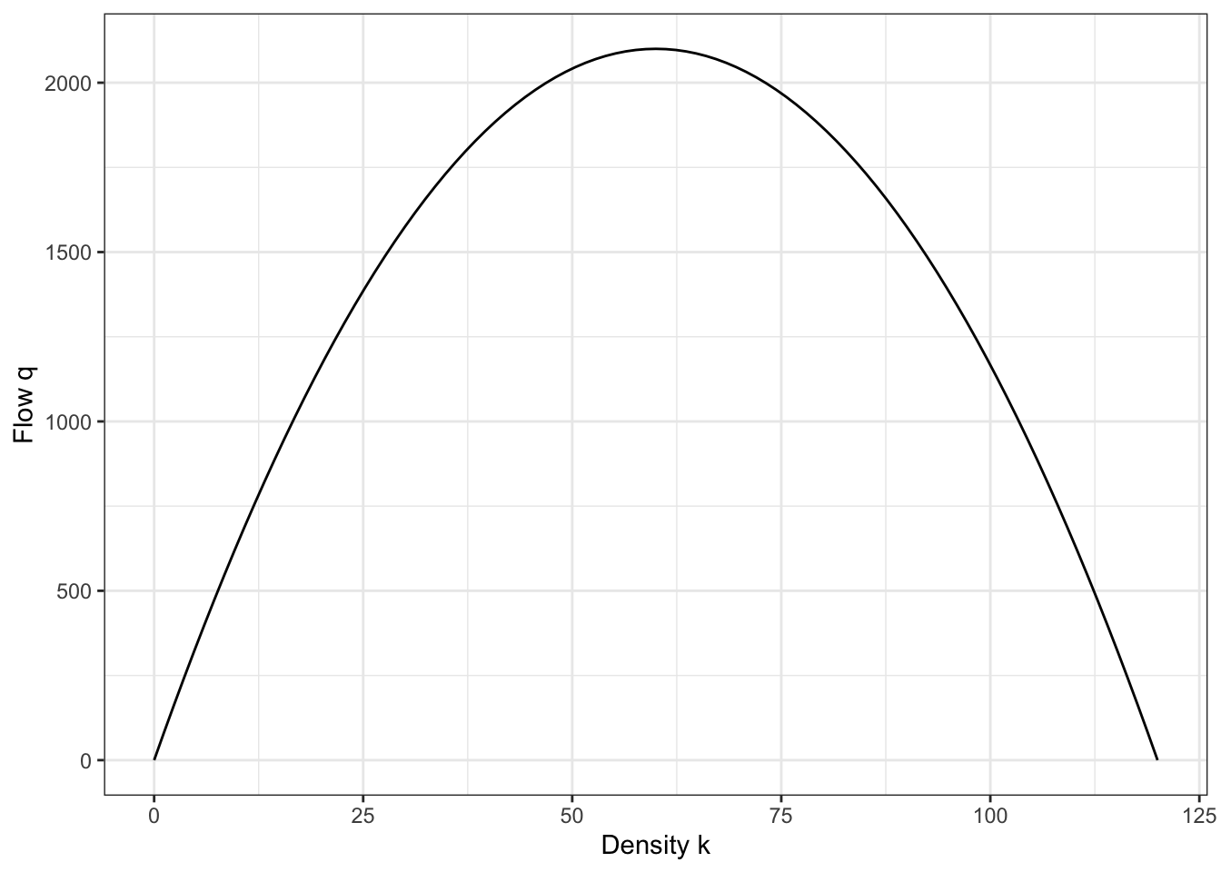
That the Greenshields flow-density model is a parabola suggests also that there is some optimal density, \(k_{opt}\) that results in a maximum flow rate, \(q_{max}\). This point happens where \(dq/dk = 0\).
\[\begin{align} q &= v_f k - v_f k^2/k_j \\ \frac{dq}{dk} = 0 &= v_f - 2 v_f k / k_j\\ \end{align}\] \[ k_{opt} = k_j / 2 \tag{2.14}\]
Placing Equation 2.14 into Equation 2.13:
\[\begin{align} q_{max} &= v_f k_{opt} - v_f k_{opt}^2/k_j \\ &= v_f k_j/2 - v_f \frac{k_j^2}{4k_j} \\ \end{align}\] \[ q_{max} = \frac{v_f k_j }{4} \tag{2.15}\]
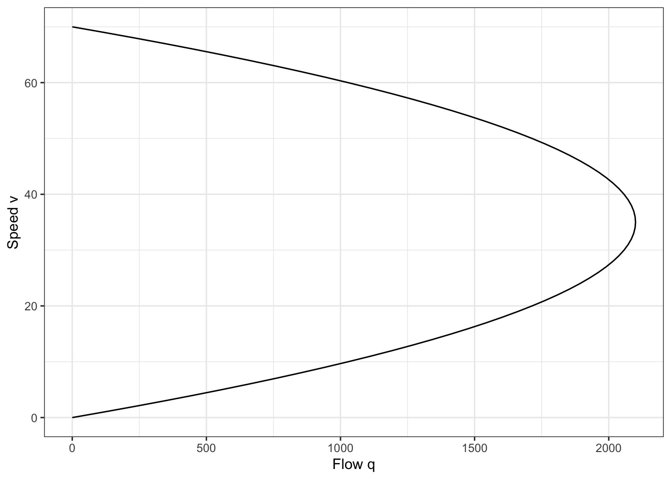
Beginning again with the speed-density model in Equation 2.12, we can make the other substitution, \(k = q/v\). This leads to a parabolic relationship between speed and flow,
\[ q = v k_j - v^2 k_j/v_f \tag{2.16}\]
Figure 2.9 shows this modeled speed-flow relationship. As before, the optimal speed is \(v_f/2\) and the optimal flow rate is \(v_f k_j / 4\).
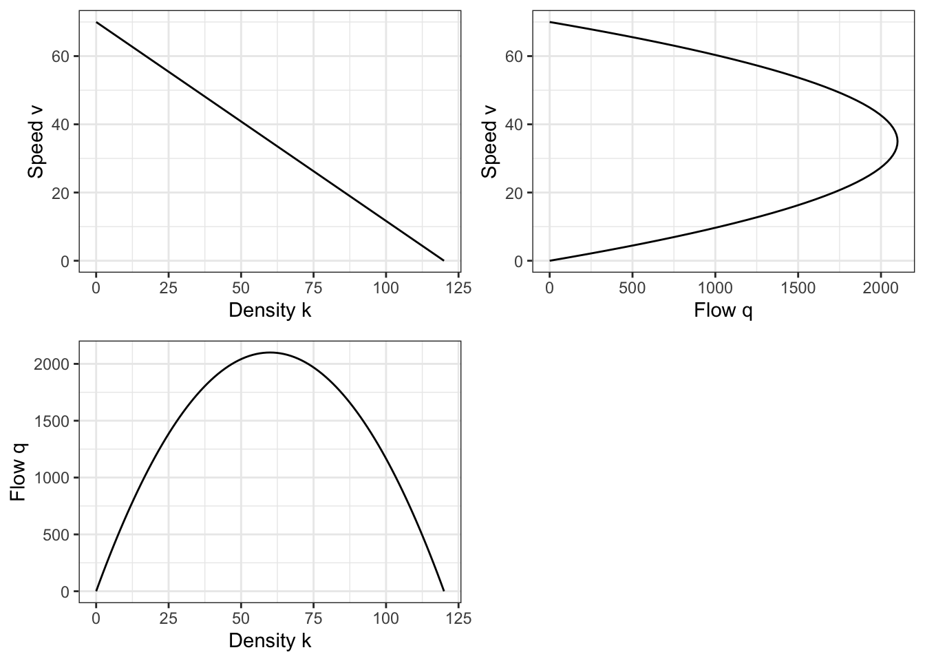
Together, the three models for speed-density, flow-density, and flow-speed form what is called the fundamental diagram of traffic flow theory. The fundamental diagram for the Greenshields model is shown in Figure 2.10, and allows an analyst to identify for a given speed or density observation what the flow rate and other parameters are likely to be.
How well does this model represent actual roadway performance? Figure 2.11 shows the Greenshields model fundamental diagram imposed on speed, flow, and density data collected on GA-400 north of Atlanta, Georgia (Ni, 2015). Each point represents a 15-minute period where the researchers collected the average speed, density, and flow rate on the roadway.
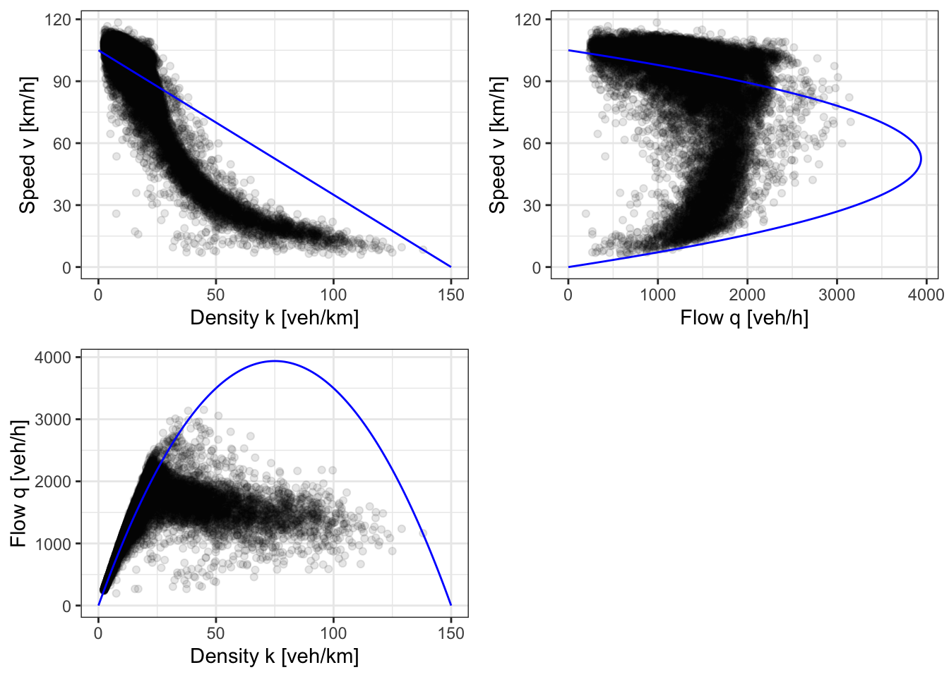
Clearly the Greenshields model is limited; engineers in practice will use more complicated theoretical models, techniques developed from empirical observations, or simulations. But there are a few key points that the Greenshields model illustrates that are common to traffic behavior in general:
- Traffic flows at a maximum speed when uncongested.
- As density increases, the speed decreases gradually at first, and then suddenly.
- When the speed decreases suddenly, this results in a sudden decrease in the flow rate.
2.3 Microscopic Traffic Flow
Frequently, engineers need to design crosswalks, left-turn signals, and other smaller systems rather than just free-flowing highways. The macroscopic models presented in Section 2.2 are not really appropriate for this, so we need to look at a smaller scale.
If an event — like a vehicle passing a point on a road — occurs randomly and independently with a rate \(\lambda\), Simeon Denis Poisson (1781-1840) showed that the probability of \(n\) events occurring in a period \(t\) is equal to \[ P(n;t) = \frac{(\lambda t)^n e^{-\lambda t}}{n!} \tag{2.17}\] As either the rate of arrivals \(\lambda\) or the time period \(t\) increases, the probability of seeing \(n\) arrivals increases, as shown in Figure 2.12.
Mathematically, the probability that zero events occur in a period is the same as the probability that the time between events exceeds a certain amount \(T\), \[ P(t > T) = e^{-\lambda t} \tag{2.18}\]
Note that Equation 2.17 gives a discrete probability. Frequently, engineers need to consider the probability that a number falls above or below a particular value. The probability that a count will exceed a discreet number \(N\) is simply one minus the cumulative probabilities less than or equal to that number, \[ P(X > N; t) = 1 - \sum_{n=0}^{N}\frac{(\lambda t)^n e^{-\lambda t}}{n!} \tag{2.19}\]
2.4 Highway Capacity Analysis
The theoretical models introduced in Section 2.2 give a tool for understanding how highways perform at different densities, speeds, and flow rates. In practice, engineers who are evaluating or designing traffic facilities will often use the Highway Capacity Manual (HCM), a publication of the Transportation Research Board. HCM analysis is based on two key concepts:
- Level of Service (LOS): The quality of operations experienced by highway users. This is described using a letter scale of A, B, C, D, E, and F.
- Capacity: The maximum hourly flow rate of a facility. This is the same concept as the theoretical \(q_{max}\) described in Equation 2.15, but the HCM is based in empirical results rather than theory.
The HCM contains methods to evaluate these two values — Capacity and LOS — for multiple transportation facilities including freeways, urban arterials, signalized and unsignalized intersections, local roads, and even transit and pedestrian facilities. In this class we will focus on basic freeway segments.
Warning 2.1: Notation
I have tried to use consistent notation throughout this chapter, with \(q, k, v\) representing flow rate, density, and speed respectively. In this section, I am using the notation that appears in the HCM, with \(V, D, S\) representing the volume, density, and speed respectively.
2.4.1 Level of Service
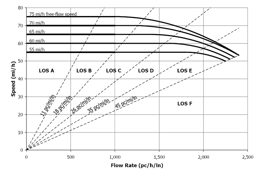
LOS for freeway segments is based on the density of the traffic stream. At low densities, drivers can easily make whatever lane changes they care to; at high densities, their speeds and movements are relatively constricted. Figure 2.13 re-creates a figure from the HCM (which in turn is a representation of Figure 2.9. Below 11 passenger cars per mile per lane, the traffic is said to operate “at LOS A.” Above a density of 45 passenger cars per mile per lane is “at LOS F.”
Note 2.1: Interpreting Level of Service
The LOS system in the HCM looks like a grade scale from a school class, but it should not interpreted that way. The goal of traffic engineers is not to always improve the LOS in the way that students always try to improve their grades. A freeway operating at LOS D or E in the peak period will be closest to its optimum throughput.
In spite of this, many cities and states have set policies mandating a minimum LOS C, mistakenly believing that this is an “acceptable” grade. What might be the consequence of these policies?
2.4.2 Capacity
For some roads, determining their capacity is straightforward: just count the cars, and find the highest hourly flow rate. But what if the road doesn’t have enough demand (yet) to hit its capacity? Or what if the road hasn’t been built yet? The HCM specifies a methodology to calculate the capacity of a road, and estimate its LOS for different traffic streams. This methodology is based on consensus and statistical relationships developed through many empirical studies, and is regularly updated based on new research.
As you can see in Figure Figure 2.13, the capacity of a road is a function of its free flow speed (FFS). As in Section 2.2, the FFS is the prevailing speed of vehicles on the road when the density is low. If the road exists, FFS should be measured. But if this is impossible, FFS can be estimated as: \[ FFS = BFFS - f_{LW} - f_{LC} - (3.22\times TRD^{0.84}) \tag{2.20}\] where
- \(BFFS\) is the base free flow speed: 75.4 mph for freeways, or speed limit + 5 mph for multilane highways.
- \(f_{LW}\) a lane width factor given in Table 2.4: if the lanes are narrower than 12 feet, people will tend to drive more slowly.
- \(f_{LC}\) a lateral clearance factor given in Table 2.5: if the shoulder to the right of the road is narrower, people will tend to drive more slowly. This factor is lessened if there are more lanes on the road.
- \(TRD\) the total ramp density of the segment: this is the number of on ramps and off ramps per mile. If no information is given, use \(0.5\).
| Average Lane Width (ft) | Reduction in FFS, $f_{LW}$ (MPH) |
|---|---|
| $w \geq 12$ | 0.0 |
| $12 > w \geq 11$ | 1.9 |
| $11 > w \geq 10$ | 6.6 |
| Lanes in 1 Direction | ||||
|---|---|---|---|---|
| Right-Side Lateral Clearance (ft) | 2 | 3 | 4 | 5 |
| $\geq$ 6 | 0.0 | 0.0 | 0.0 | 0.0 |
| 5 | 0.6 | 0.4 | 0.2 | 0.1 |
| 4 | 1.2 | 0.8 | 0.4 | 0.2 |
| 3 | 1.8 | 1.2 | 0.6 | 0.3 |
| 2 | 2.4 | 1.6 | 0.8 | 0.4 |
| 1 | 3.3 | 2.0 | 1.0 | 0.5 |
| 0 | 3.6 | 2.4 | 1.2 | 0.6 |
Once we have FFS, we can estimate the capacity of the road (in units of passenger cars per hour per lane) using the equation below:
\[ c = 2200 + (10 \times (FFS - 50)) \tag{2.21}\]
This is not the end of the analysis, however. We have determined the supply of roadway space based on an idealized traffic stream, and now we need to evaluate how the real demand for traffic fits into that capacity. The demand for traffic is the anticipated hourly volume, adjusted for peaking and variety in the traffic stream. The adjusted volume is therefore: \[ V_p = \frac{V}{PHF\times N \times f_{HV}} \tag{2.22}\] Where
- \(V\): Peak hour volume, or the hourly volume you are looking to evaluate.
- \(PHF\): the peak hour factor compensates for the peaking of traffic within an hour (see Equation 2.2).
- \(N\): the number of lanes.
- \(f_{HV}\): a heavy vehicle factor.
Note that the units of Equation 2.21 are passenger cars. Most traffic streams contain a mix of vehicles including transit buses, freight tractor-trailers, motor homes, and other heavy vehicles. These vehicles occupy more than one passenger car of space on the roadway, and perhaps even more on terrain that is hilly. The \(f_{HV}\) is calculated as \[ f_{HV} = \frac{1}{[1+P_T(E_T-1)]} \tag{2.23}\] where
- \(P_T\) is the proportion of heavy vehicles on the road
- \(E_T\) is the passenger car equivalent of heavy vehicles. This depends on the terrain of the segment, as given in Table 2.6
| Terrain | $E_T$ |
|---|---|
| Level | 2 |
| Rolling | 3 |
We now have demand volume and capacity. If \(V_p > c\), the demand exceeds capacity, and just about the only thing we can determine is that the road is at LOS F. But presuming that \(V_p < c\), we can estimate the quality of traffic flow in terms of speed, density, and ultimately LOS.
Observe the speed-flow relationships in Figure 2.13. The traffic flows at FFS at a number of different flow rates, but as the flow rate passes a certain point, the operating speed begins to decline. The flow rate where speed transitions from a constant FFS to a function of flow rate is called the break point \(BP\), and can be calculated as \[ BP = 1000 + 40 \times (75 - FFS) \tag{2.24}\] If the demand flow rate \(V_p < BP\), then the road operates at FFS. But if \(V_p > BP\), then we can calculate the operating speed as \[ S = \begin{cases} FFS - \frac{(FFS-\frac{c}{45}) \times (V_p-BP)^2}{(c-BP)^2} &\mathrm{when} &BP < V_p \leq c \\ FFS &\mathrm{when} &V_p < BP \end{cases} \tag{2.25}\]
With the speed \(S\) (or \(v\)) and flow rate \(V_p\) (or \(q\)), we can apply the fundamental flow equation to estimate the density \(D\) as \[ D = \frac{V_p}{S} \tag{2.26}\] The LOS can be obtained directly from Figure Figure 2.13 for a given density.
As a note, Equation 2.22 can be rearranged to determine the number of lanes necessary to maintain a particular LOS, \[ N = \frac{V}{(MSF_i)(PHF)(f_{HV})} \tag{2.27}\] where the adjusted demand has been replaced by a maximum service flow rate, or the maximum passenger car equivalent flow rate that would result in a particular LOS. A table of maximum service flow rates is given in Table 2.7
| Free flow speed (mph) | A | B | C | D | E |
|---|---|---|---|---|---|
| 55 | 600 | 990 | 1430 | 1900 | 2250 |
| 60 | 660 | 1080 | 1560 | 2010 | 2300 |
| 65 | 710 | 1170 | 1630 | 2030 | 2350 |
| 70 | 770 | 1250 | 1690 | 2080 | 2400 |
| 75 | 820 | 1310 | 1750 | 2110 | 2400 |
2.5 Crash Rates
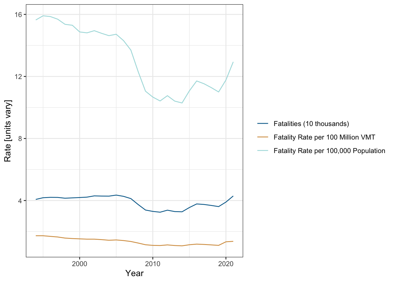
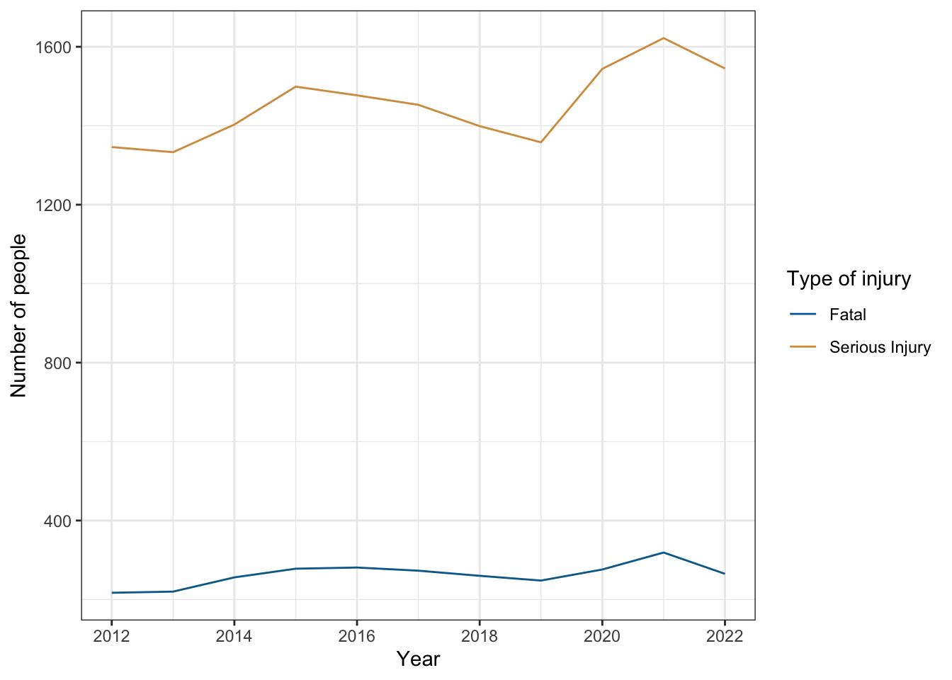
About 40,000 people die in vehicle crashes every year in the United States. Figure 2.14 shows the overall fatalities in each year as well as how this rate compares against the total population and the amount of miles driven on roadways. In general fatality rates have been dropping, primarily as a result of better vehicle engineering and government mandates for safety equipment, better roadway design, and other factors. But vehicle crashes remain a major safety hazard, and are the leading cause of death for most Americans below the age of 35. Scores of thousands of others are hospitalized with serious injuries sustained in vehicle crashes. And in recent years, data suggests that fatal and serious injury crash rates are actually rising (see Utah data in Figure 2.15).
In common speech, many people refer to vehicle crashes as “accidents” implying that they could happen randomly without explanation. Similarly, media outlets frequently use passive voice to describe vehicle crashes, e.g. “A family died on I-15 this morning when their car rolled over.” Both of these uses of language serve to remove people and engineers from their role as agents in the crash; all crashes have a cause rooted in driver error, poor roadway design, or both. This is not to say that people are always to blame for their own crashes; often times the error and carelessness of others cause harm and destruction that people cannot avoid. But being careful about how we as engineers describe vehicle crashes will help in accepting our need to identify problem spots and solutions.
Tip 2.2: Who is really at fault?
A driver on a rural road with a 55 mile per hour speed limit does not see a sign telling him that the speed limit has been reduced to 25 miles per hour upon entering a town, because the sign was obscured by an overgrown bush. No other roadway design elements tell him that he should lower his speed. The driver strikes and kills a pedestrian because there wasn’t enough distance or time for him to stop at his high speed.
In this case, law enforcement will usually assign blame to the driver. Sometimes they’ll even assign it to the pedestrian! But how much of the blame should go to the engineers who designed and maintain the road? What design elements could have prevented this crash, or helped the driver know to lower his speed?
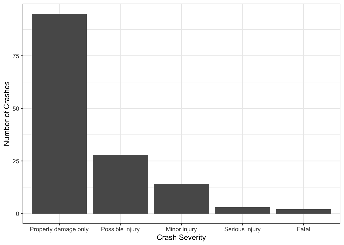
Of course, most crashes do not result in fatalities. Every jurisdiction will have slightly different laws describing crash severity; Figure 2.16 shows the distribution of three years of crashes by severity for a road in Provo. Most crashes are property-damage only, meaning that vehicles or objects along the road might be damaged, but no people reported injuries. Others involve injuries of varying severity, and some involve fatalities.
The Highway Safety Improvement Plan (HSIP) is a federal program to improve safety that state agencies must apply to federal aid roads in order to get transportation funding. A related reference published by AASHTO to help agency engineers implement the HSIP is the Highway Safety Manual (HSM). The HSM lays out several steps that engineers undertake to evaluate and improve highway safety:
- Network Screening: Which roads — roadway segments or intersections — have elevated crash rates relative to other segments or intersections?
- Diagnosis: For areas with elevated crash rates, what kinds of crashes are most prevalent? Is there an obvious causal factor for many of the crashes?
- Select Countermeasures: Based on the diagnosis, are there any elements of the roadway that could be improved? Signs added, trees removed, or roads realigned?
- Economic Appraisal: What is the cost of the countermeasures, and what is the prospect for them to alleviate crashes?
- Prioritize Projects: For all potential countermeasures, which ones are most necessary to implement immediately? Which can wait?
- Safety Effectiveness Evaluation: After the countermeasures are installed, how much do they lower crash rates?
In this class, we will mostly consider methods pertaining to step 1 and step 4.
2.5.1 Network Screening
2.5.1.1 Crash rates at an intersection
Most crashes occur in or around intersections, where drivers have to negotiate maneuvers with right-of-way, and where the paths of vehicles are in conflict with each other.
Tip 2.3: Conflict points
Draw all the potential vehicle paths at a typical four-sided intersection. At how many points do these paths cross each other? Each of these conflict points represents a potential place for a crash if a motorist does not understand or does not follow the rules of the intersection.
Engineers typically calculate the crash rate at an intersection as a rate per million entering vehicles. So to calculate this value for an intersection for a year, we apply the following equation:
\[ RMEV = \frac{\mathrm{crashes\ in\ a\ year}}{\mathrm{approach\ AADT}\times 365} \times 10^6 \tag{2.28}\]
One tricky element of this equation is that AADT is often given as a two-way volume, and this equation is for entering vehicles. This may mean you need to halve the AADT for a road to calculate the correct rate.
2.5.1.2 Crash rates on a segment
Some crashes do happen on roadway segments unrelated to an intersection. These are somewhat more rare, and might happen at various points along a segment that is several miles long. So, engineers use the crash rate per hundred million vehicle miles on roadway segments (or locations more than 100 feet from an intersection):
\[ RHMVM = \frac{\mathrm{crashes\ in\ a\ year}}{AADT * 365 * \mathrm{length\ in\ miles}}\times 10^8 \tag{2.29}\]
2.5.1.3 Crash rate critical values
The rates introduced in the previous sections do not help us determine whether the rates are unusually high for similar roads in the region. To do this, we need to compare the calculated rates among multiple roadway segments. The \(z\)-score of a observation \(i\) is an indicator of how unusual it would be to find an observation at least that large if it were part of the same normal distribution as other observations. The \(z\) score for a single observation is defined as
\[ z_i = \frac{x_i - \bar{x}}{\sigma_x} \tag{2.30}\]
where \(\bar{x}\) is the mean value of the set of all observations, and \(\sigma_x\) is the standard devation. Recall from statistics that a \(z\) value greater than 1.645 represents fewer than 5% of observations on the standard normal distribution. We can state a hypothesis using this critical value and rearranging Equation 2.30):
\[\begin{align*} h_0&=x_i \leq 1.645\sigma_x + \bar{x} \\ h_a&=x_i > 1.645\sigma_x + \bar{x} \end{align*}\]
2.5.2 Economic Appraisal
It is worth asking what it would take to build a transportation system in which no one ever died. Surely, it would not have traffic signals, because people could run those and kill someone – all intersections would need to be grade-separated interchanges. It wouldn’t have very high speed limits: the survivability of a crash at 15 miles per hour is near 100%, and at 50 miles per hour is considerably lower especially if you collide with someone who isn’t in a car of their own. Driving would be outlawed during snow storms and heavy rains, because that is when car tires are most likely to lose their grip on the pavement. In fact, it’s probably better to not have amateur drivers. Or even cars at all.
Setting aside the questionable realism of the scenario described above, safety improvements to civil infrastructure cost money. In essence, society has made the decision that some amount of risk to life and property is acceptable. So then, how can we make a decision as to whether a particular suggested improvement is worth the cost of implementing the improvement? Specifically, what is the benefit / cost ratio of the improvement?
The benefits of safety improvements mostly come from avoiding the cost of vehicle crashes. The HSM suggests average values for the societal cost of various types of crashes, which are presented in Table 2.8 (recreated from HSM Table 7-1). These values include the cost of ambulances, medical care, property damage, lost productivity, and other similar costs. They explicitly do not include wrongful death or dismemberment damages resulting from civil court findings.
| Collision Type | Costs [2021 Dollars] |
|---|---|
| Fatal | $6,293,973 |
| Disabling Injury | $339,120 |
| Evident Injury | $124,030 |
| Fatal / Injury Combined | $248,374 |
| Possible Injury | $70,493 |
| Property Damage Only | $11,618 |
So then, how many crashes will be avoided with the new improvement? The HSM defines a method to calculate the crashes prevented at an intersection or on a segment as \[ \mathrm{Predicted \ Crashes} = \mathrm{Expected\ Crashes} * CMF * \frac{\mathrm{Forecast\ AADT}}{\mathrm{Base\ AADT}} \tag{2.31}\]
where \(CMF\) is the crash modification factor for the proposed improvement. These reduction factors can be calculated by observing crash rates before and after improvements in other places, and default values representing many studies are gathered in the HSM.
A \(CMF\) will be a number between zero (for a very effective improvement) and one (for an ineffective improvement)3 Note that multiple improvements — each with their own \(CMF\) — might be planned for a single intersection or roadway segment. In this case, the total \(CMF\) value is the product of the individual \(CMF\) values, \[ CMF = CMF_1 \times CMF_2 \times \ldots \times CMF_i \tag{2.32}\]
Occasionally, engineers use or report a crash reduction factor instead of a crash modification factor. These are related as \(CMF = 1 - CRF\). Using a \(CRF\) in Equation 2.31 will result in the expected reduction in crashes instead of the predicted number of crashes. Additionally, a \(CMF\) in practice will vary by type of crash, crash severity, and other more specific details.
Homework
HW 2.1: Headways
| Vehicle | Time of arrival (seconds) | Time to travel 100 ft (seconds) |
|---|---|---|
| 1 | 4.58 | 1.07 |
| 2 | 11.48 | 0.98 |
| 3 | 16.25 | 1.03 |
| 4 | 22.09 | 1.19 |
| 5 | 29.81 | 0.99 |
| 6 | 34.93 | 0.82 |
The timestamps and time to travel one 100-foot portion of road for 6 vehicles is recorded in the table above. Find the average time headway for these vehicles.
HW 2.2: Traffic flow rates and headways
| Count ID | Start Time: H:M:S | End Time: H:M:S | Number of Vehicles | Flow Rate VPH | Average Time Headway |
|---|---|---|---|---|---|
| A | 8:00:00 | 8:28:00 | 715 | - | - |
| B | 13:06:18 | 13:24:42 | 382 | - | - |
| C | 17:08:30 | 17:22:30 | 634 | - | - |
A study on northbound State street through Provo counted vehicles at three separate times, with the volumes and times recorded in the table above. Find the flow rate and average time headway for each of the three time periods.
HW 2.3: Peak Hour Factor
| Period | Flow Rate [vph] |
|---|---|
| 4:30 - 4:35 | 1380 |
| 4:35 - 4:40 | 1200 |
| 4:40 - 4:45 | 1740 |
| 4:45 - 4:50 | 1730 |
| 4:50 - 4:55 | 1260 |
| 4:55 - 5:00 | 1840 |
| 5:00 - 5:05 | 1630 |
| 5:05 - 5:10 | 1730 |
| 5:10 - 5:15 | 1530 |
| 5:15 - 5:20 | 1830 |
| 5:20 - 5:25 | 1940 |
| 5:25 - 5:30 | 1630 |
| 5:30 - 5:35 | 1840 |
| 5:35 - 5:40 | 1390 |
| 5:40 - 5:45 | 1230 |
| 5:45 - 5:50 | 1360 |
| 5:50 - 5:55 | 1760 |
| 5:55 - 6:00 | 1680 |
The table above contains the traffic flow rate of a road in 5 minute intervals.
- When does the peak hour begin and end?
- What is the peak hour volume \(V\)?
- What is the fifteen-minute maximum volume \(V_{15}\)?
- What is the Peak Hour Factor (PHF)?
HW 2.4: Turning Movement Counts
Conduct a turning movement count study at a signalized intersection near you.
- Select a signalized intersection with a reasonable amount of traffic; anything involving University Avenue, State Street, or University Parkway will likely have too many vehicles to count correctly. The intersections along 700 North are usually appropriate.
- Count in pairs; one student should mark the northbound and westbound approaches, while the other marks the southbound and eastbound approaches. Even though you can work in teams of two, each student MUST TURN IN THEIR OWN ASSIGNMENT (not one for the team)
- Count for four 5-minute periods (20 minutes total). During each period, mark the number of vehicles that turn left, right, and straight during each period. Also count the number of pedestrians who cross each leg of the intersection in each period. Although it would be best to do a full hour of data, this will give you a feel for the variability of data during your count.
- Summarize your counts in the 5-minute intervals followed by a total for the entire 20 minutes. Calculate a Peak Hour Factor (PHF) for the intersection the 20 minute time period using the 20 minute total as \(V\) and the highest 5-minute count as your \(V_{15}\). Note that the PHF is for the entire intersection, not each approach.
- Calculate hourly flow rates based on your 20 minute counts to flow rate in vehicles per hour (vph) in your final results.
For your final results show the flow rate (vph) for all movements at the intersection (include your counting partner’s data as well). Use that to calculate the total flow rate (vph) and percent of each turning movement on each approach. Include the PHF for the intersection with the counts (only one PHF for the entire intersection).
HW 2.5: Speed Distributions
The file at homework-speed85.csv contains 100 observed vehicle speeds in miles per hour. Using this data, answer the following questions:
- Find the 85th percentile speed for this road.
- If this were a table of 100 mean speeds — that is, each number in the table is the time mean speed observed in a 15-minute period — is it possible to find the 85th percentile speed? Why or why not?
HW 2.6: Speeds and Average Speeds
| Vehicle Number | Time of arrival (seconds) | Time to travel 100 ft (seconds) | Speed (mph) |
|---|---|---|---|
| 1 | 4.24 | 1.13 | - |
| 2 | 13.84 | 1.05 | - |
| 3 | 19.45 | 1.12 | - |
| 4 | 26.78 | 1.23 | - |
| 5 | 28.14 | 0.99 | - |
| 6 | 38.03 | 0.83 | - |
From the travel time data in the table above:
- Find the speed in miles per hour for each vehicle across the segment
- Compute the space mean speed for these vehicles in miles per hour
- Compute the time mean speed in miles per hour
HW 2.7: Density and Flow Rate
A motorcyclist on I-15 can see a 0.83 mile section of freeway in front of him. He counts 19 vehicles using the 4 Northbound lanes. Traffic was moving at a rate of 76 mph at the time. Traffic was distributed evenly over the 4 Northbound lanes.
- Calculate the vehicle density per lane on that section of the I-15 (not including the motorcyclist).
- What was the flow rate for that section of the I-15 (all lanes)?
HW 2.8: Using Lane Occupancy
There is a loop detector on University Avenue with an effective length of 7.4 feet. During peak hour traffic, it indicates that there is a total apparent presence time of \(t(p)= 821\) seconds. The average speed for the 1,419 rush hour vehicles was 43.2 mph.
- What is the apparent presence time per vehicle for the peak hour traffic?
- What is the average length of vehicle for the peak hour traffic?
- What is the apparent and actual occupancy of the road?
- What is the density of traffic on the road?
HW 2.9: Speed Study
Equation 2.6 is supposed to tell engineers how many data observations they need to collect, but the equation requires assumptions including the standard deviation \(\sigma\) and the margin of error \(E\); how can an engineer know what the standard deviation in speeds is before they collect the speed data? And how much does the calculated number of samples \(N\) depend on these assumptions?
- Calculate the number of required samples \(N\) for estimating the 85th percentile speed with 95% confidence using Equation 2.6 for a range of values for \(\sigma\) (0.2 to 5 mph) and \(E\) (1 to 3). Present these numbers in a table or a plot organized by \(\sigma\) and \(E\)
- What does your evaluation of \(N\) in part A mean intuitively? How important are these assumptions?
HW 2.10: Using Greenshields Model Equations
One hundred periods with average measurements of speed \(v\) (miles per hour) and occupancy \(o\) (proportion time occupied) from I-15 are recorded in the file at homework-Greenshields.csv. Note: Use R, Excel, or Python — don’t do this problem by hand!
- Compute the density \(k\) in vehicles per mile for each period. Use an average vehicle length of 20 feet.
- Compute the flow rate \(q\) in vehicles per hour for each period.
- Plot the relationships between density and speed; density and flow; and flow and speed.
HW 2.11: Greenshields Model
I-15 in Utah County has a free-flow speed of approximately 75 miles per hour. If the maximum flow rate is 2350 vehicles per hour per lane, compute the expected jam density per lane under the Greenshields model and draw the Greenshields fundamental diagram for I-15.
HW 2.12: Speed-Density Relationships
The speed-density relationship for a lane on SR-361 is believed to be \[v + 2.6 = 0.001(k-240)^2\] with \(v\) in miles per hour and \(k\) in vehicles per mile. Note that this is not the Greenshields model. Find:
- The free-flow speed \(v_f\)
- The jam density \(k_j\)
- The lane capacity \(q_{max}\)
- The speed at capacity.
HW 2.13: Greenberg Model
Another theoretical traffic flow model besides Greenshields is the Greenberg model. The Greenberg model describes the speed-density relationship as \(v = v_{opt} \ln(k_j/k)\) where \(v_{opt}\) is the speed that produces the highest flow rate.
- Derive the flow-density relationship implied in the Greenberg model.
- Derive an equation for the maximum flow rate in the Greenberg model as a function of the jam density \(k_j\) and the optimal speed \(v_{opt}\)
- Assuming the optimal flow rate on I-15 is 2350 vehicles per hour per lane and the jam density is 120 vehicles per mile per lane, what is the optimal speed implied by the Greenberg model?
- Plot the fundamental diagram for the Greenberg model, and compare it with the fundamental diagram for the Greenshields model in Figure 2.11). What makes the Greenberg model more representative of observed traffic patterns than the Greenshields model? What makes it less representative?
HW 2.14: Poisson’s Model
This hw-arrivals.csv file contains the arrival times of 40 vehicles.
- What is the average arrival rate in arrivals per second for the 40 vehicles?
- Divide the arrivals data into 5-second intervals and count the number of arrivals in each interval. That is, if 4 vehicles arrive between \(t = 0\) and \(t = 5\), you would count one period of 4 arrivals for that interval. Then compute the frequency distribution of arrivals per interval. That is, if 3 of the 20 periods in your data have 4 arrivals, then you would compute \(3 / 20 = 0.15\) in the
4column. - Compute the poisson probability distribution based on your calculated average arrival rate (from part A) — pay attention to your units! That is, what is the probability of seeing 4 arrivals in a 5-second period based on the Poisson probability function with your arrival rate?
- Plot both distributions. How well does the ideal Poisson distribution fit your data?
HW 2.15: Interarrival Time
U.S. Route 189 was surveyed and the intern doing the vehicle count recorded 632 vehicles during the afternoon peak hour. A bicycle path crosses this road about midway between two parks that are one-half mile apart.
- What is the average headway between the arrivals of vehicles at the crossing?
- A typical bicyclist needs 8.1 seconds between vehicles to ride across the road safely. What is the probability that any gap between vehicles will allow the typical bicyclist enough time to cross the road?
- Your (enlightened, but maybe misled) city has decided that the average cyclist needs to have an acceptable gap 90% of the time. To what value will you have to reduce the vehicle flow rate? That is, find the flow rate in vehicles per hour such that P(0; \(\lambda*t\)) = 0.90.
HW 2.16: Level Of Service
A freeway on level terrain has three 11-ft lanes in each direction, with a 4-ft clearance space on the right side. There is no shoulder on the median side. The freeway carries a ratio of 0.17 heavy trucks within its traffic flow of \(V = 4,841\) vph in the major direction. Assume a peak hour factor of 0.9. Using the highway capacity manual process,
- What is the theoretical free flow speed?
- What is the per-lane capacity of the road?
- Compute the demand volume in passenger cars per hour per lane.
- Compute the theoretical speed of the road in miles per hour.
- Compute the effective traffic density in vehicles per mile per lane.
- What is the level of service presently on the facility?
HW 2.17: Maintaining Level Of Service
A freeway with two lanes in each direction is located on rolling hills, has 11-ft wide lanes, and a shoulder 6 feet off the right-hand lane. The traffic has a heavy vehicle share of about 0.1. The posted speed limit is 60 mph. A peak-hour one-way volume of 2,880 vehicles is observed with 850 vehicles observed in the highest 15-min period. The ramp density is 0.22 ramps per mile.
- What is the current level of service for the peak hour traffic?
- If a level of service no worse than C is desired, how many lanes are needed in each direction?
HW 2.18: Crash Rates
Over the past 3 years, there have been 9, 12, and 9 crashes on a 1.94 mile long section of University Parkway. The 2-way AADT on this section of road for the three year period is 29,274 vehicles per day. What is the annual crash rate for this section of University Parkway?
HW 2.19: Crashes at an Intersection
At the intersection of State Street and University Parkway in Orem, the four roads have AADT values of 38,472, 29,483, 28,372, and 20,927. There were 99 intersection-related crashes at this intersection in the last year. What is the crash rate?
HW 2.20: Critical Crash Rates
An engineer at UDOT is worried about the crash rate at State Street and University Parkway in Orem. She calculates the crash rates at 10 other similar intersections in Utah County, and makes the table shown below. Is the crash rate at State Street and University Parkway (calculated in the previous problem) unusually high? Use a 95% confidence interval.
| Intersection | Crash Rate [RMEV] |
|---|---|
| 300 S and University Avenue, Provo | 3.323 |
| University Parkway and University Avenue, Provo | 2.161 |
| State Street and 800 N, Orem | 2.718 |
| State Street and Center Street, Orem | 2.880 |
| State Street and 1600 N, Orem | 2.743 |
| Main Street and 400 South, Springville | 2.436 |
| State Street and Cougar Boulevard, Provo | 3.407 |
| State Street and 500 East, American Fork | 2.443 |
| US-6 and 1000 N, Spanish Fork | 3.711 |
| State Street and Main Street, Lehi | 2.462 |
HW 2.21: Crashes Prevented
A 1-mile section of road has a current AADT of 7,283 and a RHMVM crash rate of 72.4. AADT is expected to grow at a rate of 0.035 for 10 years.
- What is the expected number of crashes at this intersection in the current year?
- What is the predicted number of crashes at this intersection in 10 years if no countermeasures are built?
- If a countermeasure with a CMF of 0.81 is built, how many crashes are predicted in 10 years?
- A second countermeasure is proposed with a CMF of 0.95. How many crashes are predicted with both countermeasures in 10 years?
References
Greenshields, B. D., Thompson, J., Dickinson, H., & Swinton, R. (1934). The photographic method of studying traffic behavior. Highway Research Board Proceedings, 13.
Ni, D. (2015). Traffic flow theory: Characteristics, experimental methods, and numerical techniques. Butterworth-Heinemann.
This value is given by the data, and is not the same as the maximum hourly flow rate in ?tbl-phf.↩︎
Using a binomial probability model for the probability of zero success in 1800 tries at a success rate of 0.000123; the binomial model is not part of this class, but is often covered in basic college statistics.↩︎
The HSM actually specifies some \(CMF\) values greater than one as well, for situations that are likely to increase crash rates.↩︎