5 Multi-Modal Transportation
Recall from Chapter 1 that transportation is the movement of people and goods. To this point many of the techniques you have learned concern the movement of automobiles, which may contain people and/or goods, but they are not the same thing. When you consider different ways to move people to their activities, cars are not always the best option. Cars take up space, use lots of energy, pollute the air, and cost a great deal of money to their users. Cars of course also come with a great deal of convenience and the ability to send social signals about personality and preferences, which is why they have become so important to so many people.
In this unit we will examine non-automobile modes of transportation, including active transportation and public transit.
5.1 Active Transportation
The oldest form of transportation is walking, and it remains the most common mode of transportation in many contexts. Bicycles are about the same age as cars, and are a similarly important transportation mode in many contexts. Together, these modes (alongside skateboards, scooters, and an increasing panoply of related options) are often referred to as active transportation.
Active transportation has many benefits for individuals and society over motor vehicles. It uses less energy, and in the context of walking and biking the energy expended carries positive health benefits. The infrastructure requirements are lower, with less need to provide parking or space along the right-of-way.
Two primary obstacles exist to the widespread adoption of active transportation. The first is that without careful location choices and land use planning, destinations are sometimes too far distributed for trips to be practical walking or biking. The second is related to the first, which is that walking or biking along many streets is unpleasant or dangerous.
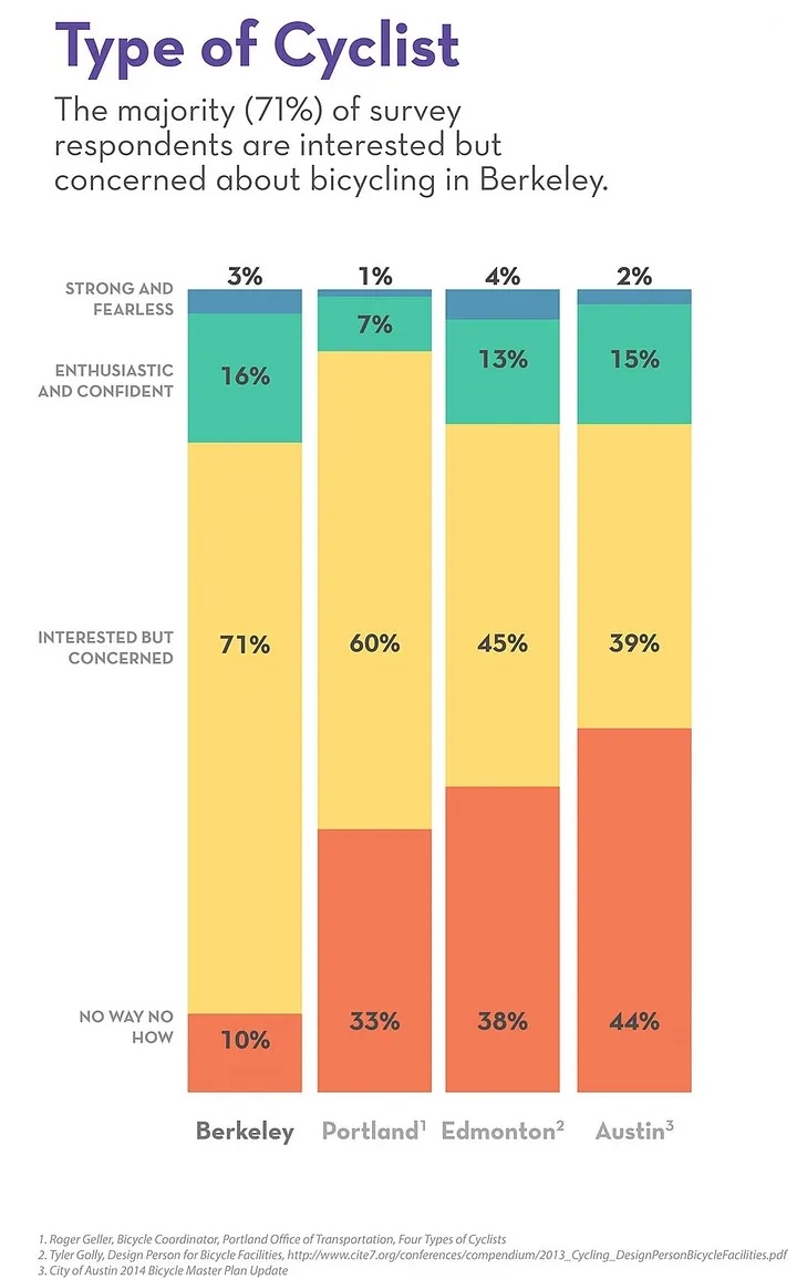
Still, active transport has sufficient benefits that many individuals ride or walk when and where they can. Transportation scholars group cyclists in particular into four categories:
- Strong and fearless cyclists ride in almost all conditions, confident in taking the lane when shoulders are obstructed or absent.
- Enthusastic and confident cyclists are eager to ride a bicycle in many contexts, but avoid difficult road conditions or trips (Dr. Macfarlane fits in this category).
- Interested but concerned cyclists would like to ride a bicycle on more of their trips, but do not because safe paths either do not exist or are not well advertised.
- No way no how individuals will not cycle under any conditions. (Dr. Macfarlane’s mom fits in this category.)
Figure 5.1 shows the distribution of cyclist types responding to surveys in many different cities. Each city is unique, but typically the largest group of people belong to the Interested but concerned category. This indicates that if more paths were available, more people would be willing to ride a bicycle for more of their trips.
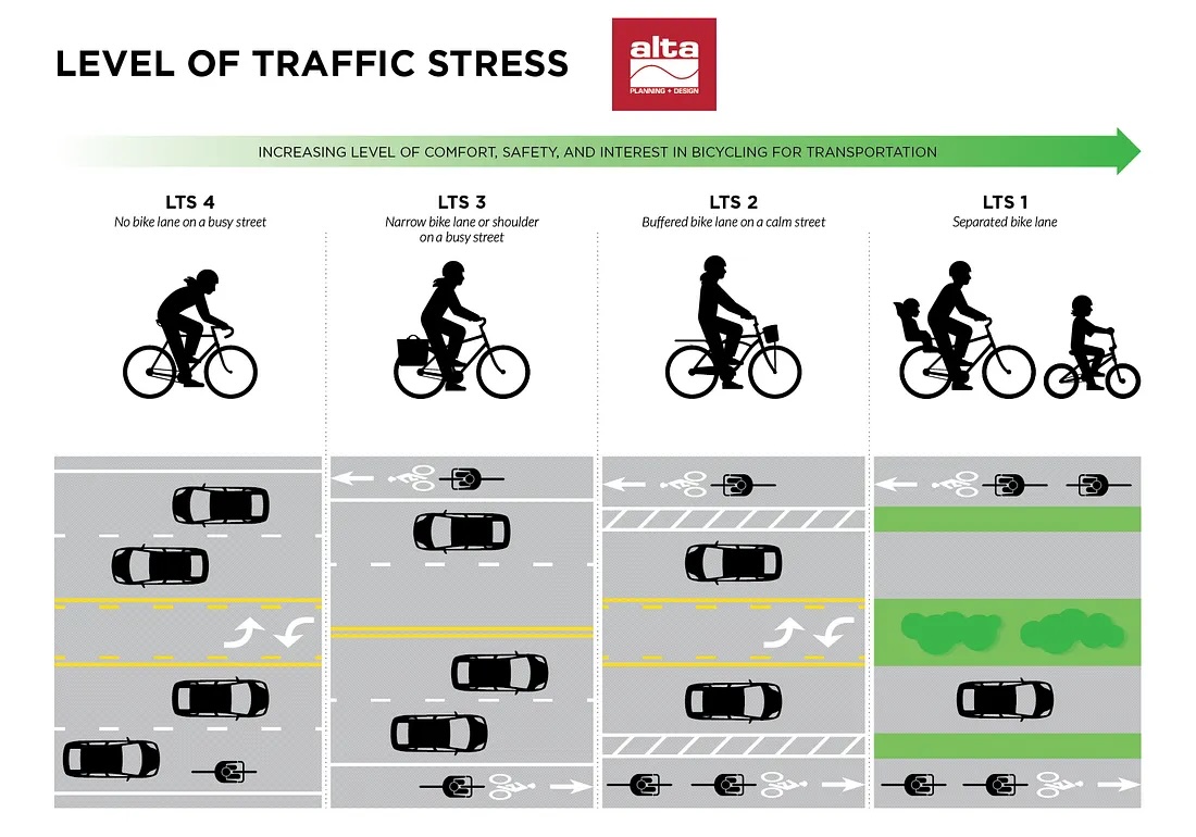
Based on these four categories, planners have developed a tool called Level of Traffic Stress (LTS) roughly identifying which kinds of cyclists might be willing to ride alongside a facility. Figure 5.2 shows LTS for varying bicycle treatments.
There is not currently a federal standard for measuring LTS. Washington State DOT has developed a scoring system for bicycle and pedestrian LTS that can be applied to almost any roadway. WashDOT additionally specifies that new projects should be built with a LTS for pedestrians and bicyclists of 1 or 2. Utah provides an interactive map of bike facilities with LTS estimates at an interactive website, https://bikeways.utah.gov/.
TipWhat kind of cyclist are you?
What kind of cyclist are you? Would you ride your bike more if the places you were going were connected by a network of roads with lower LTS?
Often, a route with sufficiently low LTS does not exist for a given trip. Sometimes it does exist, but is considerably longer. A route directness index (RDI) is the ratio of the length of the route at a desired LTS divided by the straight-line distance between the start and end points of the route.
\[ RDI = \frac{L_{LTS}}{L_{straight}} \]
Note 5.1: RDI to BYU
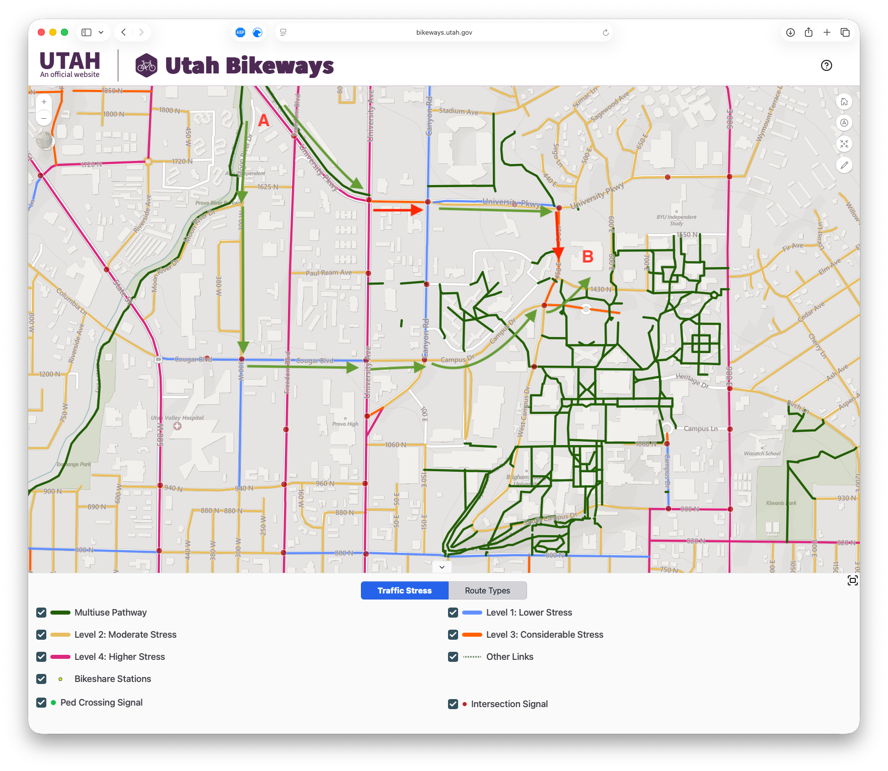
The figure below from Utah Bikeways shows the LTS for roads around BYU. What is the RDI for a route from A to B at an LTS of 2?
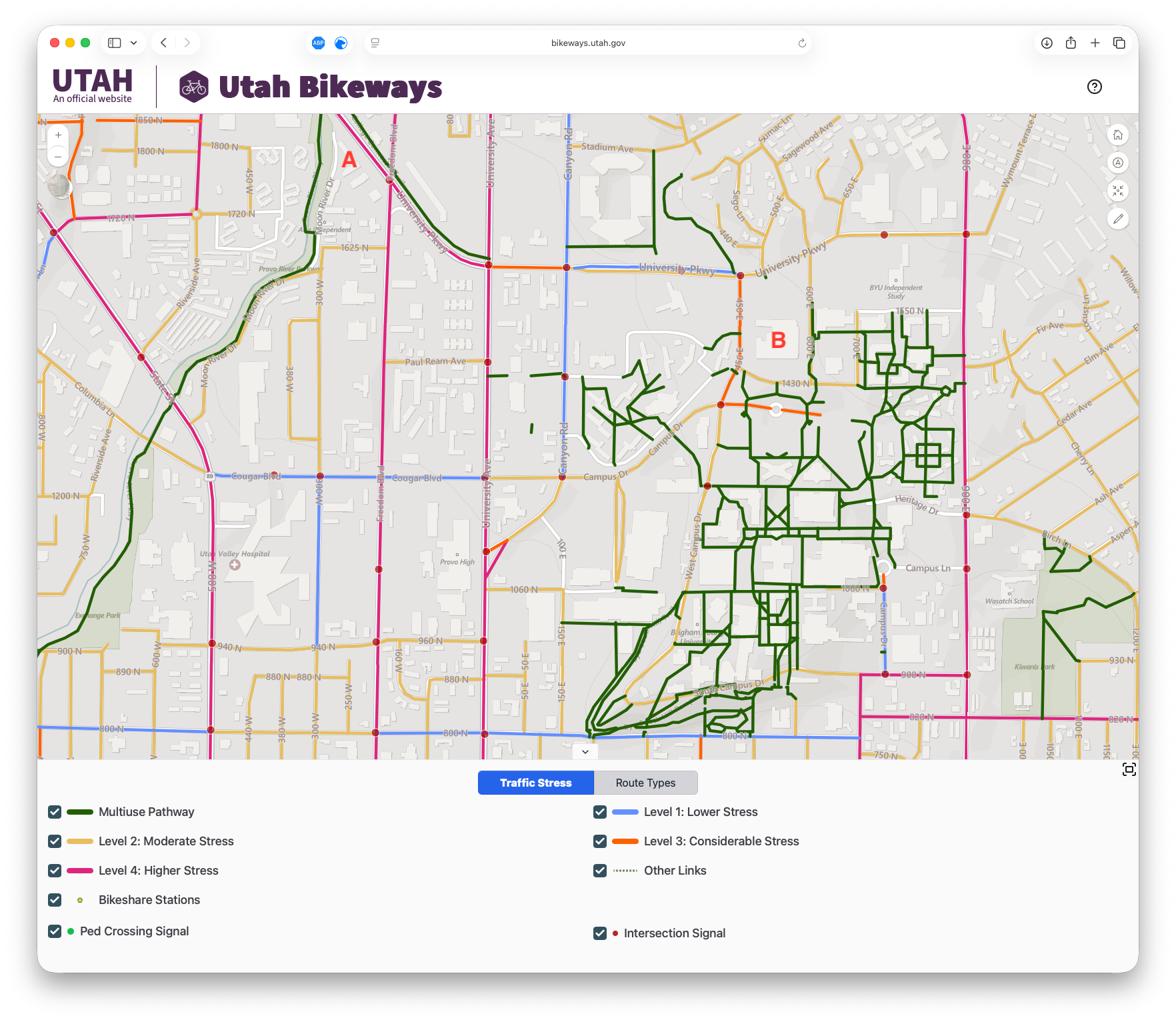
Using an online map service, the distance from A to B is 4109 feet. At any LTS, the cyclist can take a direct route up University Parkway to the Marriott Center, with a route distance of 4823 feet, or an RDI of \(4823 / 4109 = 1.17\).
But at an LTS of 2, the cyclist cannot take the direct route up University Parkway. Instead, the cyclist needs to use the Provo River Trail, 300 West, and Cougar Boulevard to get to campus. This route is roughly 7920 feet, with an RDI of \(7920 / 4109 = 1.92\).
TipImproving LTS
Note how University Parkway between University Avenue and Canyon Road is an LTS of 4, but this is a one-block section between roads with an LTS of 1 to the west and 2 to the east. This is a chokepoint, where two low LTS roads are not used as much as they could be, because they are linked with a high LTS road.
Reducing the LTS of this stretch of University Parkway to LTS 1 or 2 will almost certainly increase the number of people who choose to cycle to BYU.
5.1.1 Accessibility for All
In 1990, Congress passed the Americans with Disabilities Act, aiming to help people with different mobility needs access spaces that serve the public. The consequences of this law are far reaching for transportation agencies, and cannot be fully encompassed in this course. Rules that delineate ADA requirements are published by the US Department of Justice1 at access-board.gov. Some key highlights know:
- The ADA applies to all new construction as well as to refurbishments.
- Transit vehicles and aircraft must be accessible to people with a variety of disabilities: stop announcements have to be audible as well as visually displayed, vehicles have to be wheelchair-accessible, etc.
- Transit stations have to be accessible to people with a variety of disabilities. Fare vending machines need to have buttons in Braille, platforms need to be accessible by elevator or ramp, etc.
- Parking lots must be given sufficient accessible parking stalls, with clearance around vehicles to deploy wheelchair ramps when parked.
TipADA curb ramps on campus.
We did an in-class activity where we measured curb ramps near the WILK and the CTB. What stipulations of ADA curb ramp design surprised you? Which elements do the existing curb ramps fail to meet?
5.2 Public Transit
Public transit, generally speaking, is any form of collective transportation.2 Driving and active transportation principally use private vehicles (or no vehicle) that operate on mostly public and open roadways. Public transit, on the other hand, uses vehicles that are owned by private companies or public agencies, and people purchase a trip by paying a fare. There are many types of transit, and there are many different reasons why a region would want to include public transit in their transportation systems.
In this section you will learn how to classify and describe transit modes based on their characteristics, the benefits of public transit for the transportation system, elementary techniques in how to design and operate transit systems, and you will develop a context-specific transit plan for a community.
5.2.1 Transit Modes and Characteristics
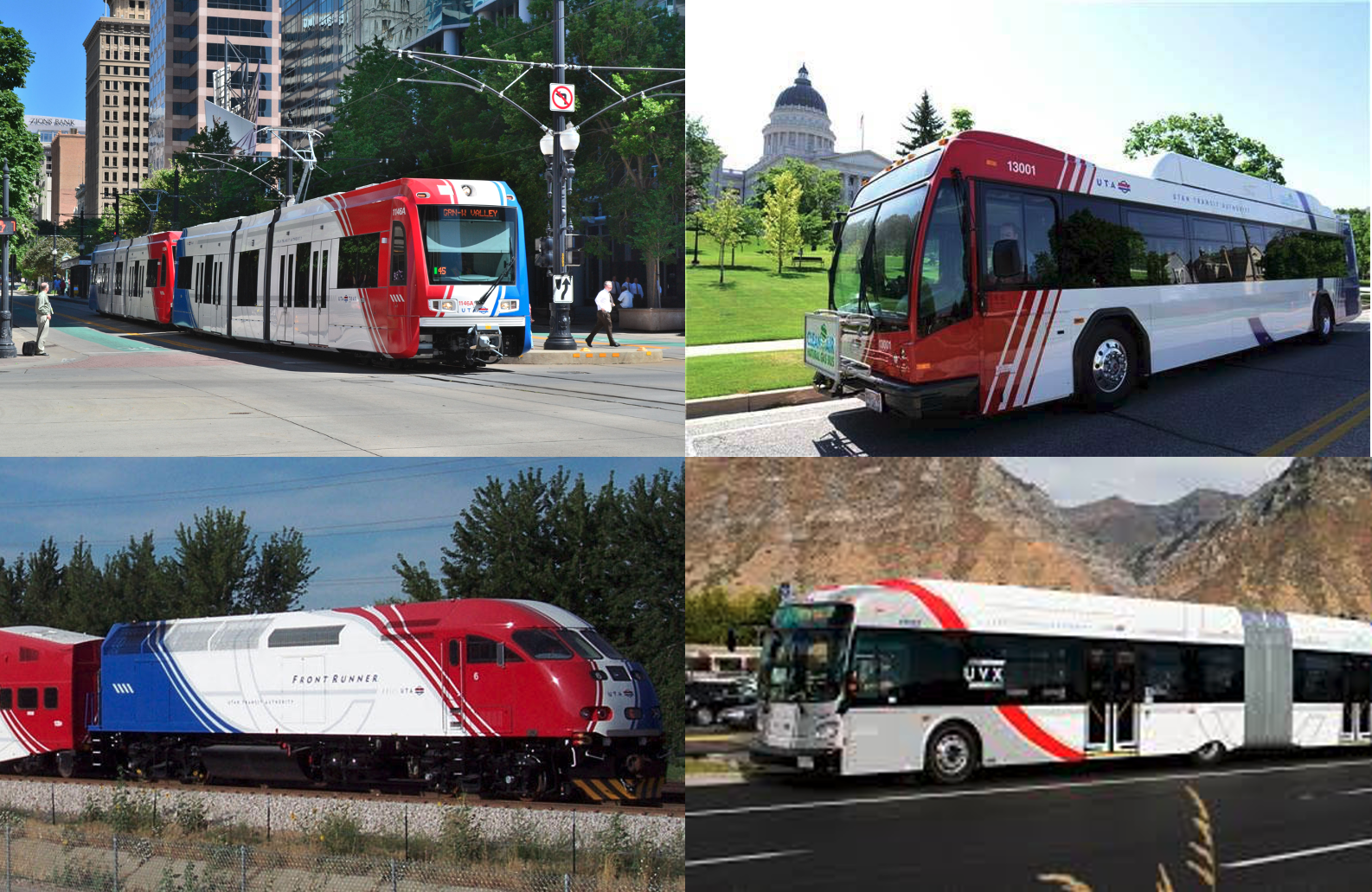
Transit comes in many different forms including buses, light rail, trolleys, taxis, funiculars, gondolas, ferries, and on and on. Some common transit modes are shown in Figure 5.3, but a complete list of all transit modes is not a simple thing to create. It’s helpful then to have a system of describing transit modes by their key characteristics. These characteristics are:
- Right-of-Way
- System Technology
- Type of Service
- Organizational Oversight
We’ll talk about each of these characteristics in turn.
5.2.1.1 Right-of-Way
Right-of-Way (ROW) describes the type of infrastructure that the transit service runs on. Many transit modes do not have a special ROW, operating in mixed traffic on public roads (like local bus services) or waterways (like ferries). These services can be relatively inexpensive, but they can also be slow if the roadways are congested. In order to improve operations, some transit services might run on separated ROW, like dedicated lanes for bus rapid transit (BRT), or intercity rail systems shared with other freight rail. Some services may even run on their own dedicated infrastructure, like gondolas on an aerial cable or an underground urban rail system.
With increasingly separated ROW the performance characteristics of the system improve, but the costs of constructing, operating, and maintaining the system increase as well. As a result, fully-controlled transit ROW is usually only constructed when demand and other conditions necessitate it.
5.2.1.2 System Technology
The technology employed by a transit service can fall into several categories.
- Vertical contact describes how a vehicle interfaces with its ROW. This can be rubber tire on pavement, steel wheel on rail, flotation, magnetic levitation, etc.
- Lateral control describes how a transit vehicle steers along its ROW. This can be a human driver using a steering wheel, or rails that guide the vehicle along a track.
- Propulsion describes how a vehicle receives power to move down the ROW. This might be a diesel engine, a diesel generator powering electric motors, or electricity received from overhead wires (catenary wire) or a third rail.
- Spacing control describes how the transit vehicles space themselves along the ROW. This can include drivers maintaining a schedule, positive train control for rail systems, or fixed spacing as on a gondola.
5.2.1.3 Type of Service
The service type of a transit system describes what kind of trips the system provides. This is akin to the mobility/accessibility discussion in Chapter 1. Three common service types are:
- Express services are designed to bring commuters from suburban areas quickly into an urban core.
- Rapid / Skip Stop services decrease overall travel time along a corridor by having widely spaced stops.
- Local services provide greater accessbility by having frequent stops, but are typically slower as a result.
Just as a combination of road types enhances the highway transportation system, a combination of transit services can help create an effective transit system. If local services are coordinated with rapid and express services, then people can experience a good balance of mobility and accessibility.
Heavier vehicles benefit from more space between stops; the time it takes to accelerate and decelerate would keep the vehicle from reaching its design speed between stops. Local bus services may have a stop on every city block. Light rail systems typically have stops every mile or so, and commuter rail systems will usually have stops every 5 miles or more.
5.2.1.4 Organizational Oversight
Transit services can be operated by various types of organizations. Jitney services are informal transit operations run by individual private operators or a coalition of them. Private taxi companies receive licenses from a state or city to operate on-demand transit services. Most larger transit agencies are connected in some form with state or local government, with governors and state legislatures having the ability to appoint board members and set laws governing the agency’s practices. In exchange for this oversight, the transit agency can fund itself with tax revenues and raise money through public bond initiatives.
5.2.2 Benefits of Public Transportation
Public transit systems can be expensive to operate, and are often complicated to design. Then why do regions build them? Some of the most important reasons include:
- Improve mobility for disadvantaged populations: Many people cannot operate private vehicles, either because they have a physical disability that prevents them from doing so; or because they cannot afford to own, insure, and maintain a vehicle; or any other number of reasons. These people use public transit as a way to travel to work, school, or other activities that they would otherwise not be able to participate in.
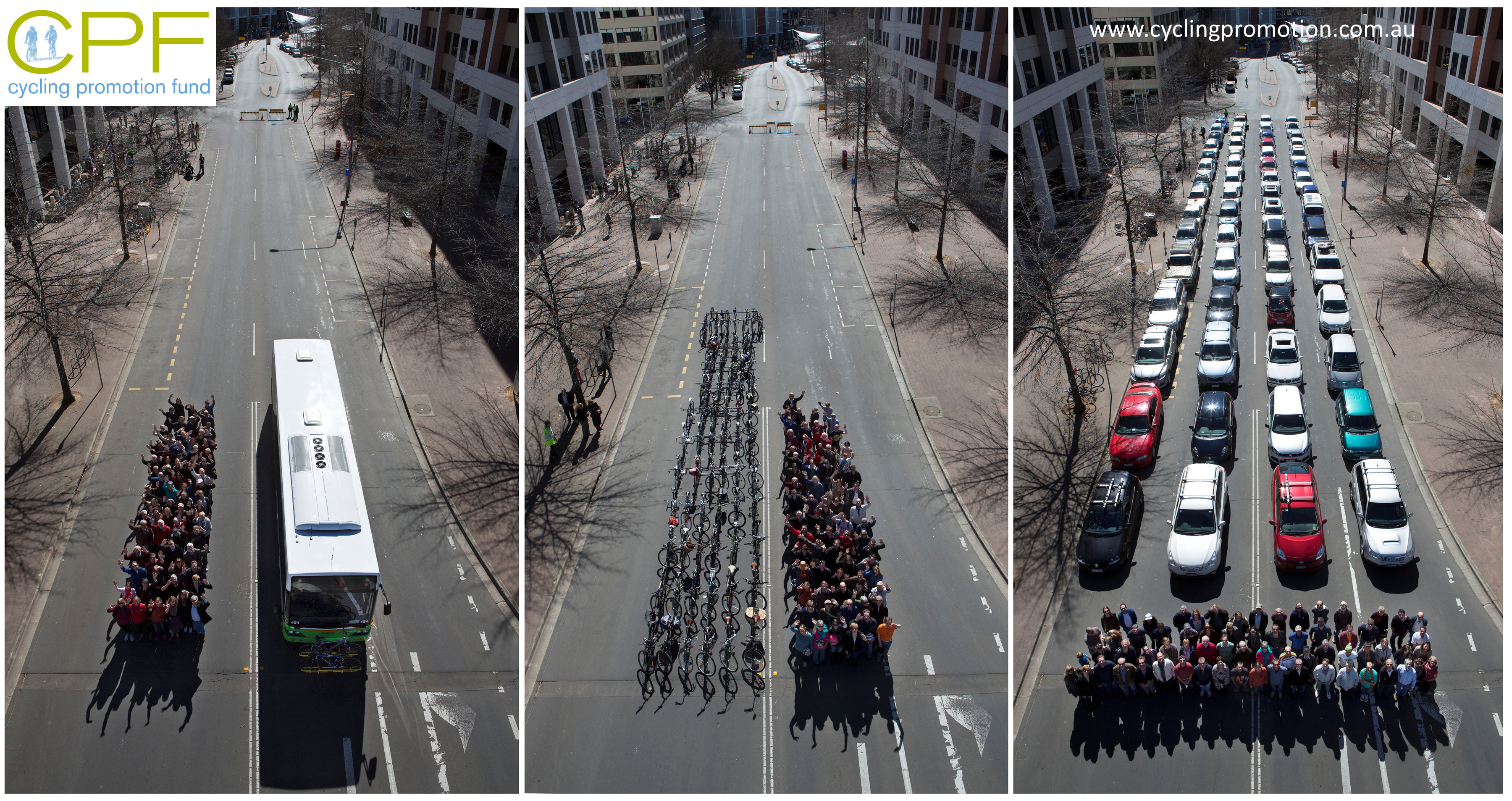
- Make better use of urban space: Personal vehicles with low average occupancy take lots of space on the roadway and in storage (parking). In places where many vehicles would want to travel, building sufficient road and parking infrastructure may be too expensive, or there are likely better uses for that space. Transit and active transportation modes are much more space efficient, as shown in Figure 5.4
- Conserve natural resources: Even though buses are large and use lots of fuel, per-passenger fuel efficiency can be substantially lower than for automobiles. Trains can be even more energy efficient because the rolling friction of steel wheels on steel rails is so much lower than rubber tires on pavement. Buses also have a much longer service life than private vehicles due to regular maintenance; local transit buses have an average service life of 12 years or 500,000 miles (Laver et al., 2007). This means that the environmental cost of manufacturing and recycling or salvaging transit vehicles can be somewhat lower than an equivalent number of private vehicles.
- Increase safety: Transit vehicles are operated by professional drivers who maintain awareness and avoid distraction much more successfully than the general population. Also, no one minds if you use your phone while riding the bus. Figure 5.5 shows the fatality rate for highway and transit modes from 2014 through 2018 using data from the Bureau of Transportation Statistics.3
5.2.3 Transit System Design and Operations
The positive benefits of transit can only be realized when people use it. And for people to use it, it has to be useful. There are seven demands of useful transit service:
- It takes me where I want to go
- It takes me when I want to go
- It is a good use of my time
- It is a good use of my money
- It respects me
- I can trust it
- It gives me flexibility in my plans
Note that transit doesn’t have to be the best mode — the fastest, cheapest, cleanest, most convenient — in order for it to be useful to a large number of people. But understanding the demands of a useful service will help engineers focus on the elements of system design that will make the most difference to transit riders. These demands can translate to design standards and performance measures, as illustrated in Figure 5.6. Some design parameters are related to more than one of these elements. We will discuss these parameters in turn.
Tip
Recall that terms listed in bold are things you should know for the test. Also for your future as an engineer.
5.2.3.1 System coverage and stop access
System coverage is the area served by a transit agency. Often, the agency will have some sort of goal to provide transit service within a quarter-mile of a certain percent of the region’s jobs or residents. This has equity implications as well; federal disability law requires that transit agencies provide paratransit service to qualifying individuals living within this coverage area.
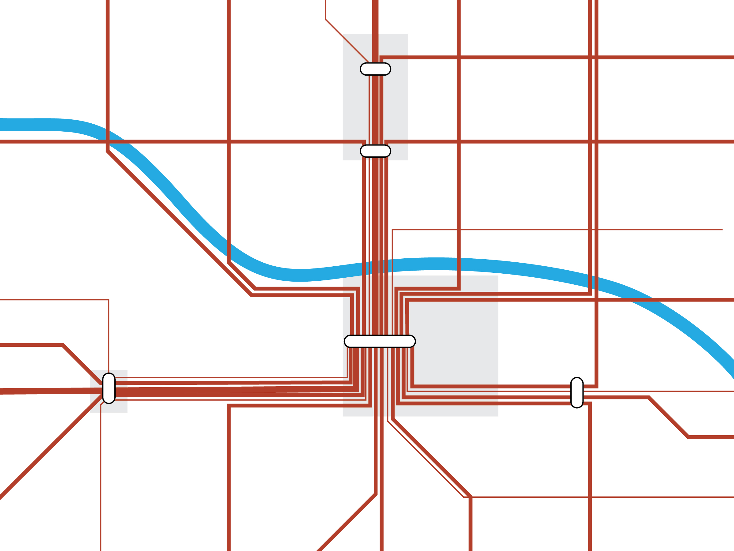
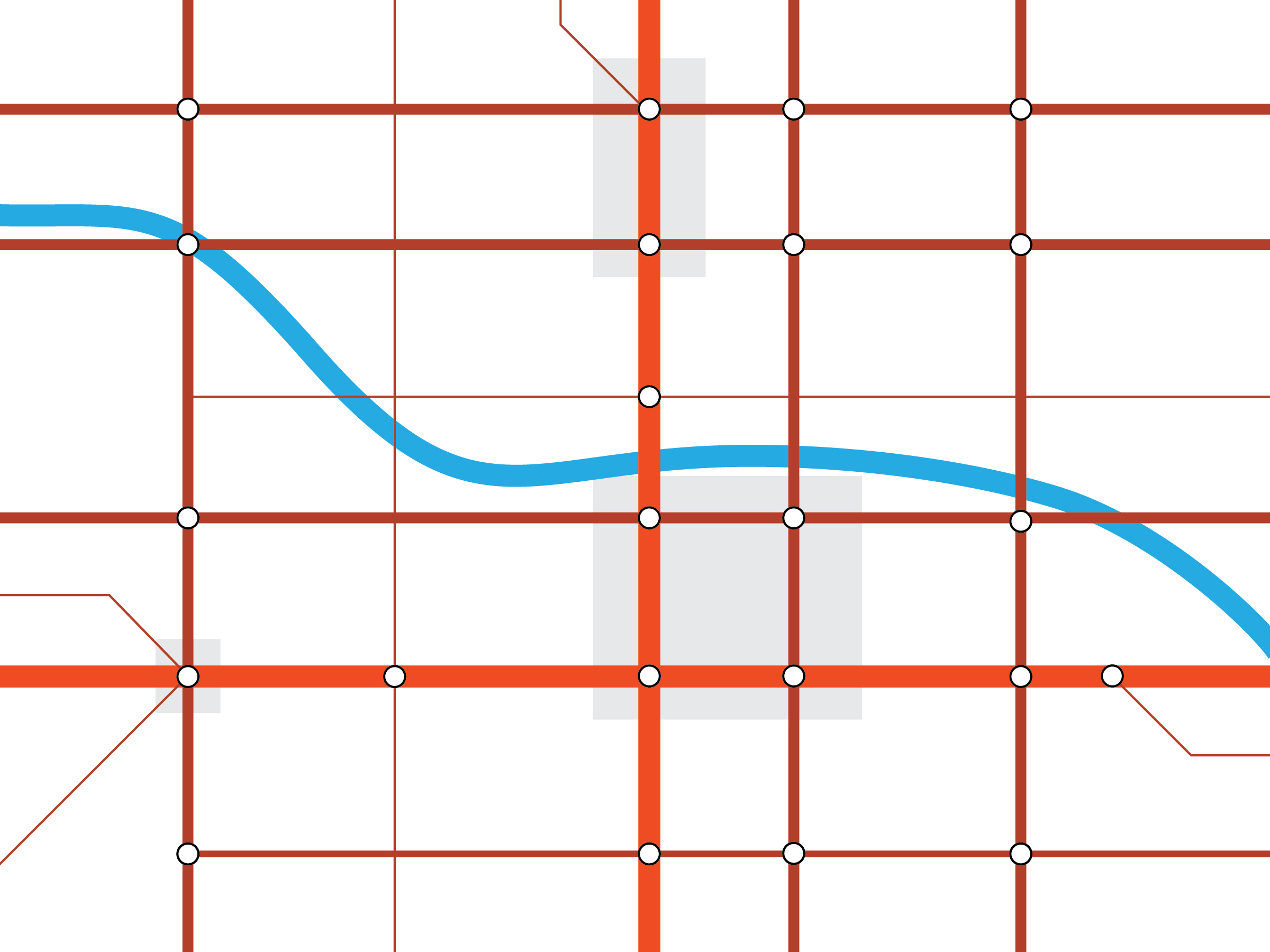
People access transit systems at defined stops or stations, served by defined routes. The effectiveness of transit is greatly enhanced by the land use surrounding the stations. Figure 5.7 (a) shows pedestrian walking times in the grid-based network of downtown Provo and Figure 5.7 (b) in the suburban dendritic (tree-like) network of Lehi. A single stop in Provo will be able to access more destinations more conveniently than a single stop in Lehi or another typical suburban area.
Other considerations that will help get transit passengers closer to their destinations include:
- Place parking lots behind buildings instead of in front of them. This way people don’t have to walk long distances across parking lots to get to the store.
- If you must design cul-de-sacs in new neighborhoods, include space for paths that will allow pedestrians and cyclists to cut through the neighborhood more directly.
5.2.3.2 Frequency and span of service
Frequency is how often a transit vehicle arrives; this is the inverse of headway. We would say that UVX has a frequency of 10 buses per hour, or that it operates on a 6-minute headway. Span of service is the number of days or hours in which the service operates. Increased frequency and span leads to reduced wait times and increased system capacity, but costs more because more vehicles, fuel, and driver hours are required.
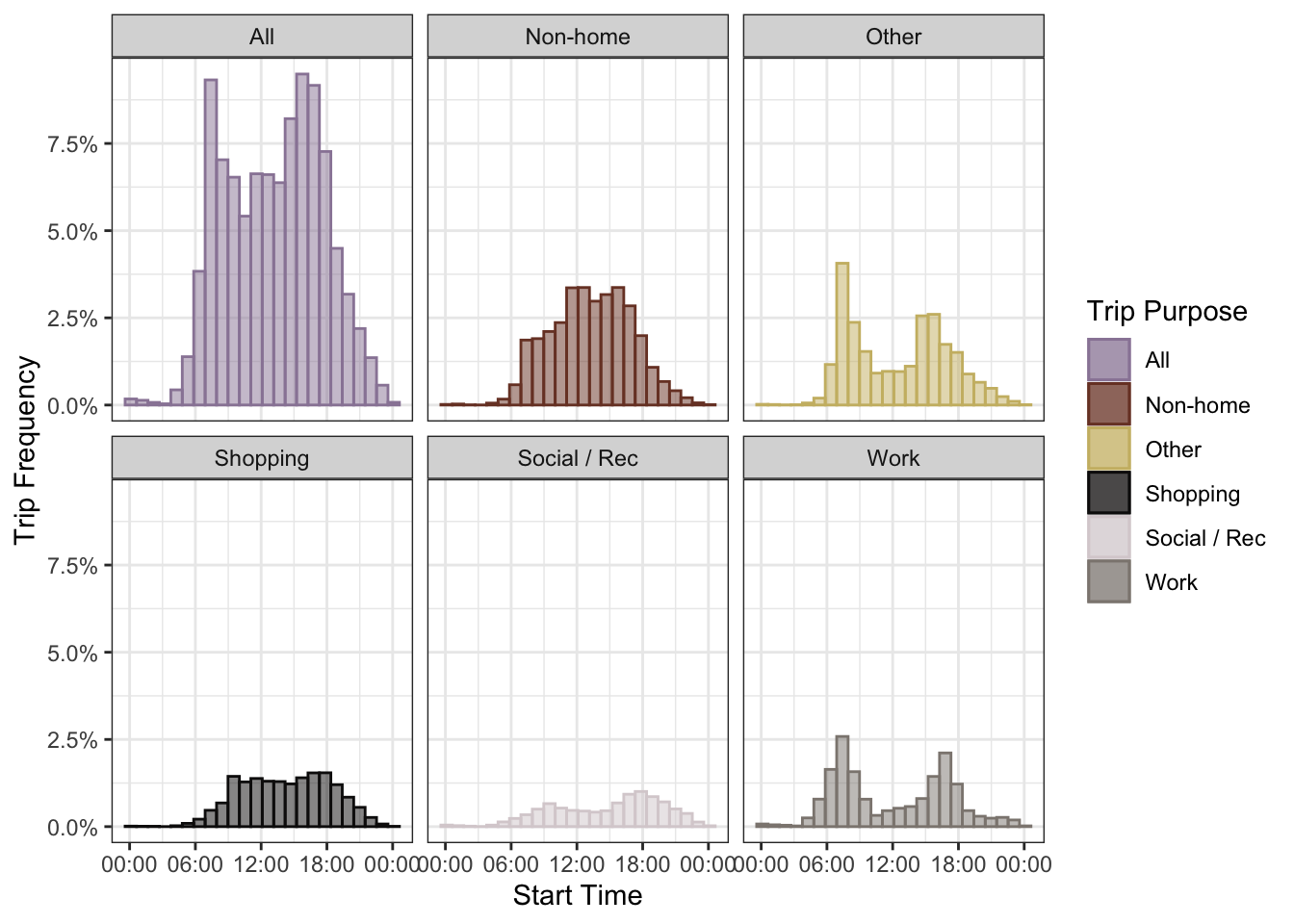
Trip-making is distributed unevenly across the day. Figure 5.8 shows the density distribution of trip start times by different trip purposes collected from the National Household Travel Survey. Many transit systems are aimed at the home-to-work trip purpose; as the figure shows, most of these trips happen during the AM and a PM “peak” period, between 6 and 9 in the morning and between 4 and 7 in the evening. Transit services will often add additional frequency during these peak periods. The home-to-work journey also makes up only a few percent of all trips in a region. They are often the longest and most regularly made, but they are not most trips.
Most people do not travel in the middle of the night. Running all-night transit services can be expensive to offer with so few trips happening. But shift work near factories or hospitals or other situations might justify running some all night services. Adding UVX, FrontRunner, and TRAX services on Sunday is an active policy debate in Utah. It is likely that such services would operate at a substantial loss, but knowing that transit is an option every day might help more people choose transit for more kinds of trips.
5.2.3.3 Speed and dwell time
The speed of transit vehicles is important in competing with other transportation modes, but it will almost always be slower than private automobiles, especially in uncongested situations. Constructing dedicated right-of-way for transit vehicles will greatly improve transit travel times, but can be extremely expensive. Giving transit vehicles priority at traffic signals — keeping a light green until the bus gets through, called Transit Signal Priority(TSP) — can also be marginally helpful and is affordable to implement.
Lots of the increase in travel time comes not from the speed of the vehicles, but the delays associated with station dwell time. Large numbers of passenger boarding and alighting the vehicle will increase the dwell time. Strategies to decrease dwell time include:
- Board and alight passengers through separate doors, and provide more doors on the vehicle
- Require fare payment cards or proof of payment so that people are not counting coins in the bus stairwell while boarding
- Elevate platforms and lower vehicle floors so that wheelchair users and other individuals can board easily and without complex wheelchair ramp deployments
It is also important to limit the number of times a transit vehicle needs to slow, stop, and re-accelerate. In general, heavier vehicles take longer to slow down and speed back up; common stop /station spacing for different modes are as follows:
- 5-10 miles between stations: Commuter rail
- 1-3 miles: Heavy rail
- 0.5-1 mile: Light Rail, BRT
- 0.25 mile: Local bus
If a system has too many stops, it will be too slow and no one will ride it. But if it has too few stops, it won’t be useful to anyone and no one will ride it. Often, transit routes will deviate from the main road to reach a destination like a school or a hospital or a seniors home. This will improve accessibility for some, but too many deviations will slow down the total travel time and discourage others. It’s usually best to have direct routes, and encourage these trip generators to locate on major roads.
Studies of how people perceive time suggest that waiting for something feels considerably longer than it actually is, on the order of two to ten times as much. That is, someone who says they waited 10 minutes for the bus probably actually waited between 3 and 5 minutes if they were not timing it carefully. This means that transit systems should be designed to minimize wait time: if you can improve the speed of a bus by 2 miles per hour or you can cut the wait time by a couple of minutes by adding another bus, get the extra bus. It’s also important to cut out transfers between routes, and give people a one-seat ride if possible.
5.2.3.4 Fares
Transit systems generate some of their operating revenues through collecting fares. The farebox recovery of transit systems in North America is usually on the order of 15-30%, with the balance coming from state and local taxes (often sales taxes).
The amount people pay for their transit trip is important. Obviously, more people will ride if transit is cheap or even free. The method people use to pay their fares matters also. Having a single fare for all trips is easy, but it makes people who use the system for short trips pay more per-mile than people who take long trips. Monthly passes are easy to use and can lower the per-trip cost for regular trip makers. Many employers and universities will pay for a transit pass for their employees or their students, making the system effective free. But people on limited incomes often cannot save the money for a transit pass, paying more expensive ride-to-ride fares. Some agencies are implementing fare capping, where riders who pay for each ride eventually ride for free after paying the equivalent monthly pass price.
Transit agencies that need to raise revenues will also lose some riders if they raise fares. Transit fare increases involve tricky questions of social equity. If a transit agency were to raise its fares, many of the people who continued using transit would be those who had no other options — often because they couldn’t afford a car. Because of this, transit agencies sometimes need permission from their state legislature to implement a fare increase.
TipThink
UVX has been free for all riders for its first few years because of a government grant. What would be the consequences if UTA were to make its entire system fare free?
5.2.3.5 Customer Experience
Transit is public transportation in every meaning of the word. This can sometimes create uncomfortable or confusing situations for some riders. Good transit agencies often take care to ensure that their drivers and other customer-facing staff are trained to provide security and be helpful in lots of different scenarios.
Other things that transit agencies can do to create positive customer experiences:
- Ensure that vehicles are well-maintained and clean.
- Ensure that stations are clean, secure, and well-lit.
- Provide restroom facilities on long-distance vehicles and at large stations, and ensure that these are clean and well-maintained.
- Design effective and easy-to read maps of the system and other informational materials.
- Translate wayfinding and informational messages into other languages (including braille) as necessary.
TipThink
Have you ever had a bad experience on transit? Is there something that the agency could have done or should have done to help your experience?
Also, it’s also important to reflect on feelings we may have against transit or transit riders that are actually rooted in inappropriate prejudice or privilege.
5.2.3.6 Reliability
Few things are more disheartening to a transit rider than being late to an important event because your bus was running behind schedule. It is even worse when you miss a bus because it was running ahead of its schedule. Transit systems need to be reliable.
A key performance measure for transit systems is its on-time performance. Generally, this is the percent of vehicles that arrive at a timepoint not earlier and not later than 5 minutes of the scheduled time. It is important to plan bus schedules carefully; sometimes vehicles will need to linger at stops so that they don’t get ahead of their schedule. This is infuriating to all involved, especially when it happens every day.
In systems with high passenger loads, a phenomenon called bunching can affect on-time performance and reliability. Bunching happens when a vehicle gets behind its schedule because station dwell times are lengthened by the high volume of boarding passengers. But the next vehicle on the route doesn’t encounter as many passengers (because they are all on the first vehicle), meaning it gets ahead of its schedule. Eventually, the two vehicles coincide, with a heavily packed bus running just a few seconds ahead of a mostly empty bus. Solutions to bunching include:
- Slow the second vehicle down to maintain proper headway, if not the schedule.
- Prevent passengers from boarding the first vehicle at a particular stop.
- Increase the frequency on the line so that passenger loads don’t get so high to begin with.
5.2.3.7 Flexibility
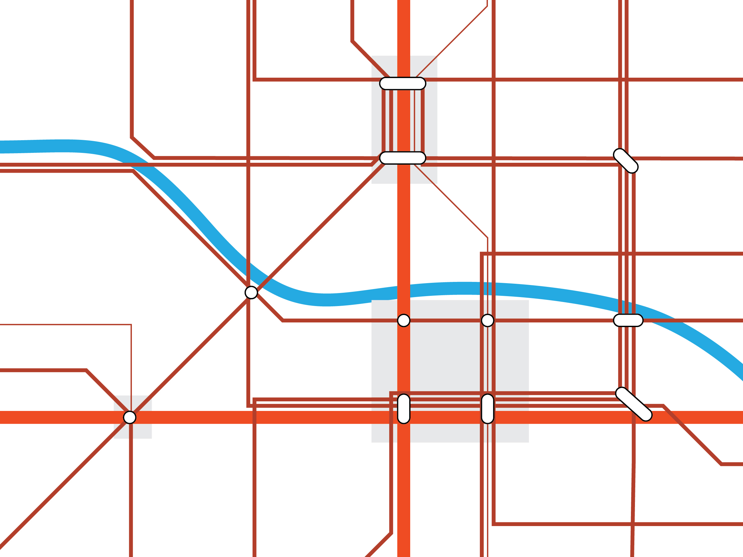
A well-designed transit network should be able to serve many different trip markets. Some of this is a function of land use: if more businesses, schools, and residents located along a transit line then transit could be used for more trips. But the transit network design matters as well: different configurations will enable different trips. Three different network design paradigms include:
- A “Multi-hub” network will focus feeder systems on a series of high-capacity transfer stations. This is the system that mostly exists in Utah, with hubs at Salt Lake Central, Provo Central, North Temple, and other places.
- A “Radial” network brings all transit routes into a more limited collection of transfer points. This works when the downtown area contains almost all transit destinations.
- A “Grid” network provides excellent coverage and flexibility, but if the frequency on the grid is not high enough, transfers can be very long and realistic paths are pretty limited.
Automobiles provide ultimate transportation flexibility, and people sometimes fear losing this flexibility if they use transit. Some of these fears can be allayed through high-frequency, long-span, and reliable service. Others could be addressed through cooperation with taxi or ridehail providers; e.g., transit agencies could reimburse Uber fares for monthly passholders who need to pick up a sick child at school.
5.3 Rail Systems
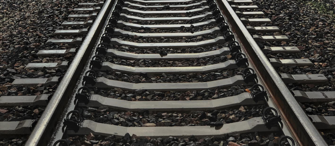
Railroads are an efficient way of moving heavy loads across distances. The steel wheels on steel rails allow for very little rolling friction, meaning that once trains have accelerated to a speed, they can coast for a long way with low energy use. The tracks are more costly to build than highways, but can last for a long time with proper design and maintenance.
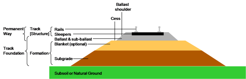
Elements of a rail foundation are shown in Figure 5.10. The steel rails are pinned to ties (or sleepers) that can be made from wood or concrete. The ties are then embedded in an aggregate ballast which sits on graded soil or aggregate placed on top of the natural soil. This design allows for the forces of the train to be distributed downwards and into the earth.
When building rail systems for transit riders, a primary consideration is the spacing between stops, and the acceleration / deceleration regimes of the rail vehicles. Is there enough space for the train to reach its top speed? Is it more efficient to maintain the top speed and then brake, or coast for a little while, saving fuel but at the expense of time? Figure 5.11 shows these regimes on a helpful speed / time diagram. The vehicle begins accelerating and when it reaches its top speed, it may either maintain that speed or coast until it needs to brake as it approaches the next station.
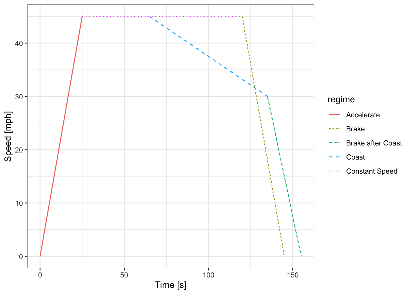
The equations that describe these regimes are derived directly from basic equations of motion, and are repeated in Table 5.1
| Time in Regime | Distance in Regime |
|---|---|
| $s_{b,c}$ is distance to brake after coasting, etc. | |
| Acceleration | Acceleration |
| $t_a = \frac{V_{top}}{\bar{a}}$ | $s_a = \frac{V_{top}^2}{2\bar{a}}$ |
| $t_{a,c} = \frac{V_{top} - V_{ec}}{\bar{a}}$ | $s_a = 0.5 t_{a,c} (V_{top} + V_{ec})$ |
| Constant Speed | Constant Speed |
| $t_v = \frac{s_v}{V_{top}}$ | $s_v = S - (s_a + s_b)$ |
| $t_{v,c} = \frac{s_{v,c}}{V_{top}}$ | $s_{v,c} = S - (s_a + s_b + s_{b, c})$ |
| Coasting | Coasting |
| $t_c = \frac{V_{top} - V_{ec}}{c}$ | $s_c = S - (s_a + s_{b, c})$ |
| $t_c = \frac{V_{top} - V_{ec}}{c}$ | $s_c = 0.5 t_c (V_{top} + V_{ec})$ |
| Braking | Braking |
| $t_b = \frac{V_{top}}{\bar{b}}$ | $s_b = \frac{V_{top}^2}{2\bar{b}}$ |
| $t_{b,c} = \frac{V_{top} - V_{ec}}{\bar{b}}$ | $s_{b,c} = \frac{V_{ec}^2}{2\bar{b}}$ |
| Dwell | Dwell |
| $t_d = P_{on} t_{on} + P_{off} t_{off}$ | $s_d = 0$ |
5.4 Freight
As introduced at the outset of these notes, transportation is the movement of people and goods. To this point many of our problems have dealt with neither of these things, but rather we have looked at how vehicles move on the roadway. In the next unit we will look at how people choose which transportation modes to use, and how to design transportation systems to maximize people throughput. But for now we will talk about goods.
Freight is the commercial transport of goods from place to place. It can be difficult to model and understand freight and freight movements, and that makes it difficult for engineers to plan for and design transportation systems to accommodate freight.
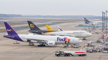
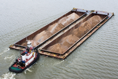
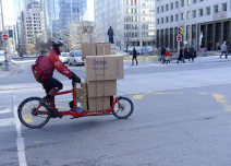
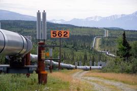
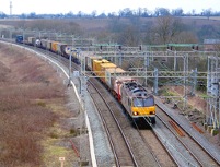
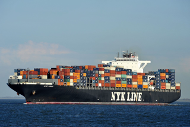
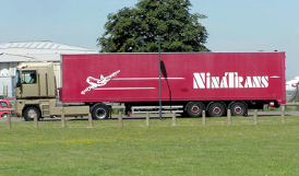
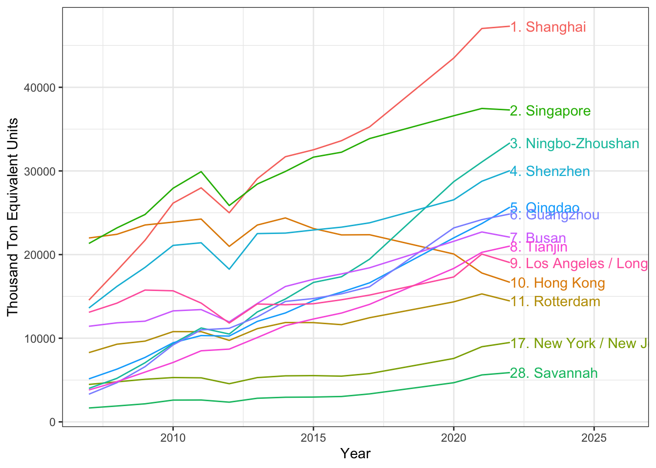
Freight uses modes that we haven’t addressed to this point, and that might be hidden from typical analysis. The Mississippi River carries more freight by weight on barges than any interstate highway. Of course, trucks usually have to get the cargo from the shipper to the barge and off again. Truck traffic that supports port and rail operations is called drayage. Some of the most common freight modes are pictured in Figure 5.12). Intermodal freight shipments became considerably easier with the invention of the shipping container, a standard metal box that can be easily moved between ships, rail cars, and truck beds with cranes and forklifts. A plot of the some of the busiest shipping ports by volume is given in Figure 5.13; most of the world’s busiest ports are in Asia, and the growth of international shipping from Asia to the rest of the world has been impressive. It is not too great a claim to say that freight containerization has been the most important technological innovation for the global economy in the last 100 years.
Contracts between freight operators and shippers are usually privately arranged and not always rational. The cost to ship a truckload of hogs from a North Carolina farm to a Wisconsin meat packer is not printed in a neat schedule of prices. So even if the average cost of shipping by rail is cheaper than truck, a shipper might have a relationship with a truck-based freight operator that leads them to pick the truck at a higher price, or a lower price that an external analyst cannot observe.
The commodities shipped as freight are all different from each other, and require different considerations for time of delivery, method of shipping, etc. Coal is cheap and heavy; electronics and pharmaceuticals are light but expensive and fragile. Produce and many food products must be refrigerated from the farm to the store, and operational inefficiencies on rail networks mean that produce in the United States rarely moves by rail.
Many freight operators are large enough to work as de facto monopolies. For passenger travel, you can sample 1% of households and get a good picture on how people get to work and back; if you sample 1% of freight companies and don’t get Union Pacific you miss a lot of goods movement. Also UPS and FedEx are different enough from each other that understanding one won’t help you understand the other.
5.5 Aviation
Air transportation is the fastest mode of transportation available for most passenger and freight trips, especially over long distances. One benefit of air travel is that it requires somewhat minimal infrastructure along the right-of-way. Airports themselves, however, are large and complex pieces of civil engineering infrastructure requiring careful design. And even in the air, aircraft and their crews are aided by air traffic control systems and radar beacons that define flight paths and elevations for the safe operation of aircraft.
5.5.1 Airline Operations
Figure 5.14 shows the annual airline passengers over time by region. Global air traffic took a big hit during the COVID pandemic, but is largely back to its pre-pandemic levels (though the chart has somewhat outdated data).
Airline passengers have different needs, and this may lead airlines to offer different kinds of services. Business travelers may need to go from anywhere to anywhere, but usually travel on weekdays and as solo travelers. Recreational travelers often travel on or near weekends, in small groups or families, and to a somewhat more predictable set of destinations. Business travelers often book travel with only a few days notice and are more sensitive to schedule, and recreation travelers often book months ahead and are very sensitive to price. These are generalizations, but they are reflected in different operations and service plan offerings from airlines.
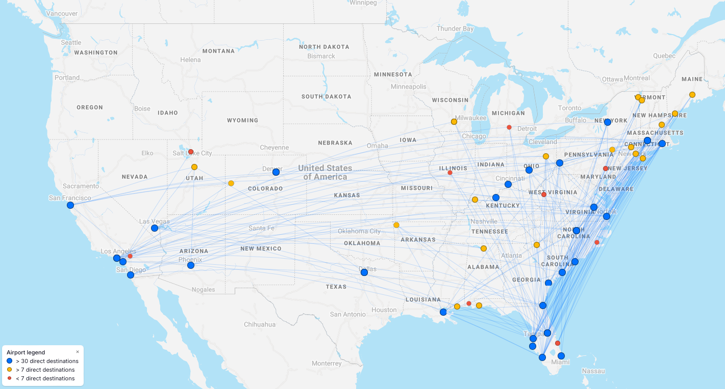
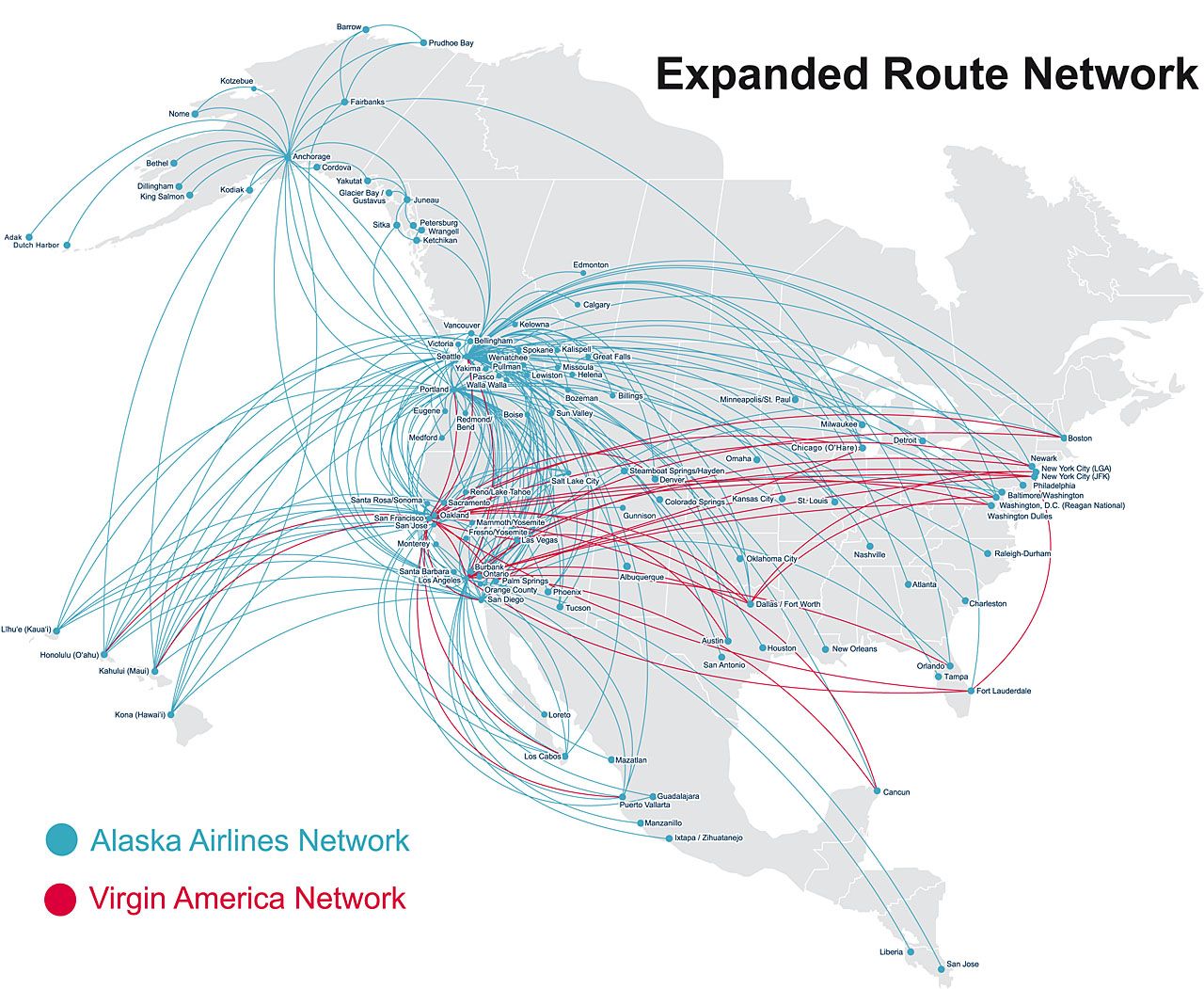
Figure 5.15 shows the route maps for two airlines that have different target audiences. Breeze Airways operates a point-to-point network that is largely constructed to help people in the northeast get to and from warmer vacation destinations. Even though Breeze serves both Pittsburgh and Louisville, it is unlikely that passengers would try to make this trip by connecting in Tampa (the flights may not even travel on the same day). Instead, Breeze tries to understand where people in Pittsburgh may want to go for their vacations and plans flight times and destinations that it believes it can serve profitably. Airlines like this will often operate a single aircraft type to save on pilot training and maintenance.
On the other hand, Alaska Airlines operates a hub-and-spoke system designed to connect travelers between most airports in the Pacific northwest. In this case, Alaska knows that it does not have enough passengers to fly from Calgary to Anchorage regularly. Instead, it operates flights between Seattle and dozens of other aiports. Its passengers need to change planes in Seattle, but the airline can serve many more potential origin-destination pairs. In this case, Alaska tries to coordinate its flights so that they arrive at Seattle to build the most origin-destination pairs. Airlines with a hub-and-spoke system often cater to business travelers, but vacation travelers fill up extra space. Airlines like this will operate multiple different aircraft types, because the needs of the Nome to Anchorage route are different from the Seattle to Los Angeles route.
TipThink
Presently, Provo (PVU) is served by point-to-point operators that make it easy to get some specific places, like Arizona or Southern California. Beginning in Fall 2024, American Airlines began daily service to its hubs in Phoenix and Dallas. Has this affected your ability to use PVU as a replacement for SLC?
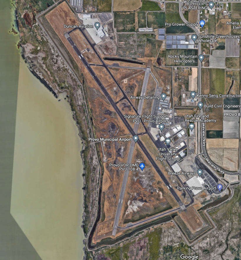
5.5.2 Airport Design
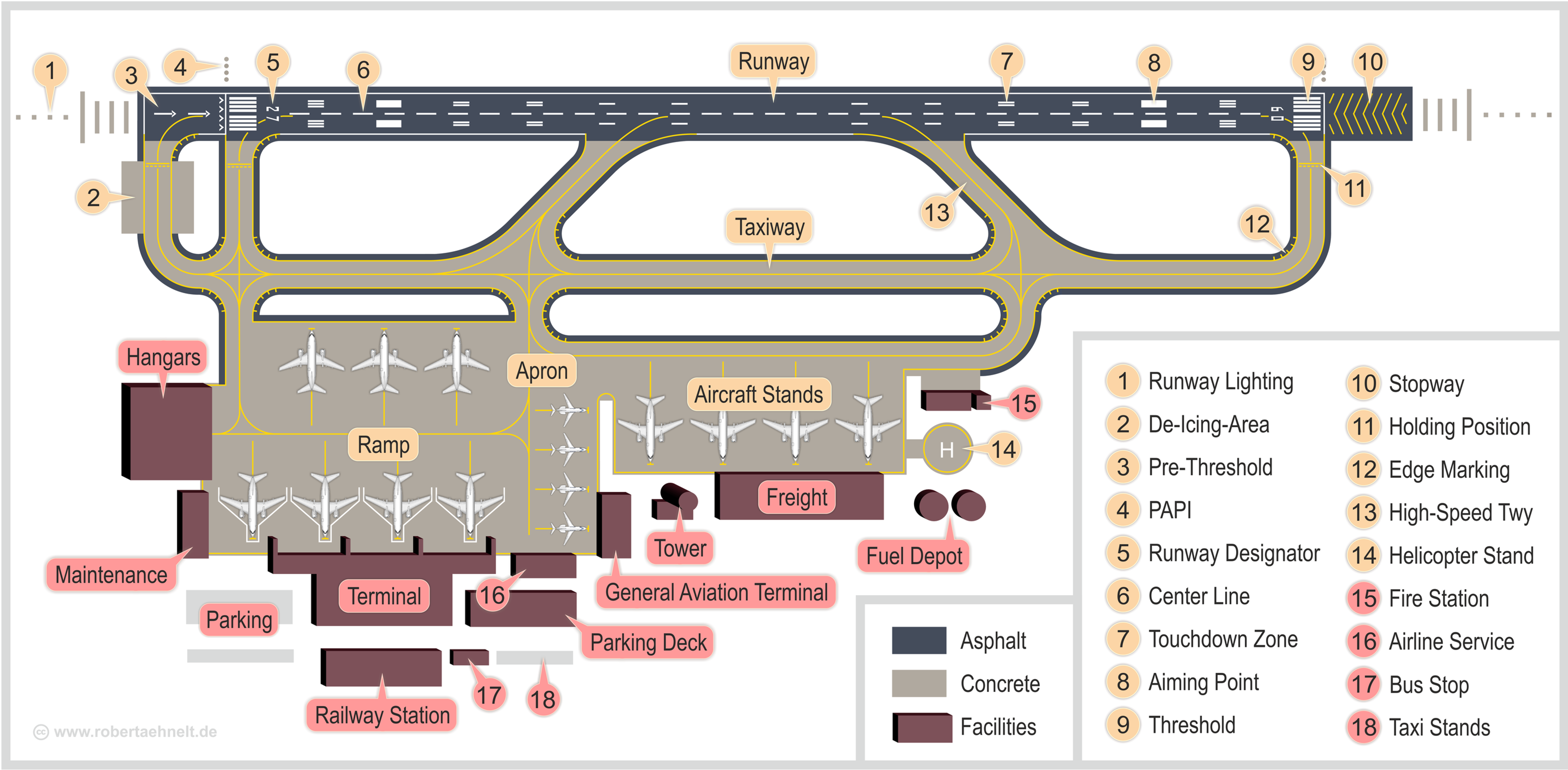
In order to effectively serve the demand for freight and passenger traffic, airports consist of several interrelated facilities or elements. These are grouped into two basic sets illustrated in Figure 5.16: landside and airside facilities. Landside elements include things such as ground transportation baggage handling, security, fuel infrastructure, and other elements related to ground operations. Airside elements include the apron, taxiway, runways, and other elements need for aircraft operations.
The design and siting of airports is a complex issue. Access to population centers and ground transportation is merely the first step. Other considerations include wind patterns, clearance on runway approaches, and noise. Many of these analyses are detailed in the FAA Advisory Circular (AC) 150/5300-13B.
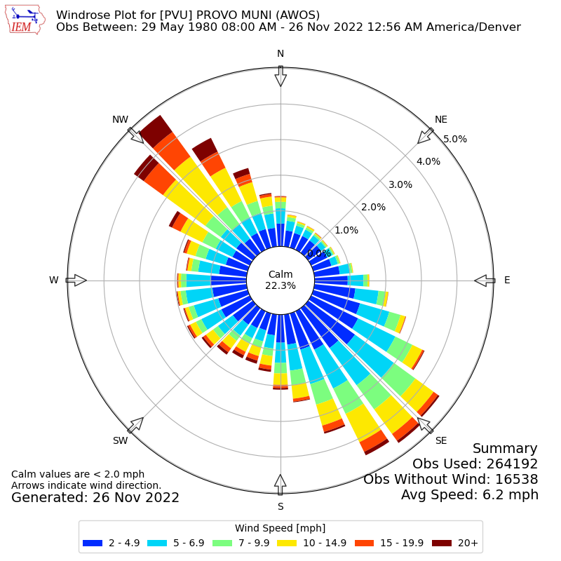
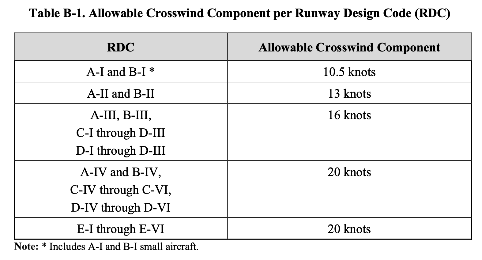
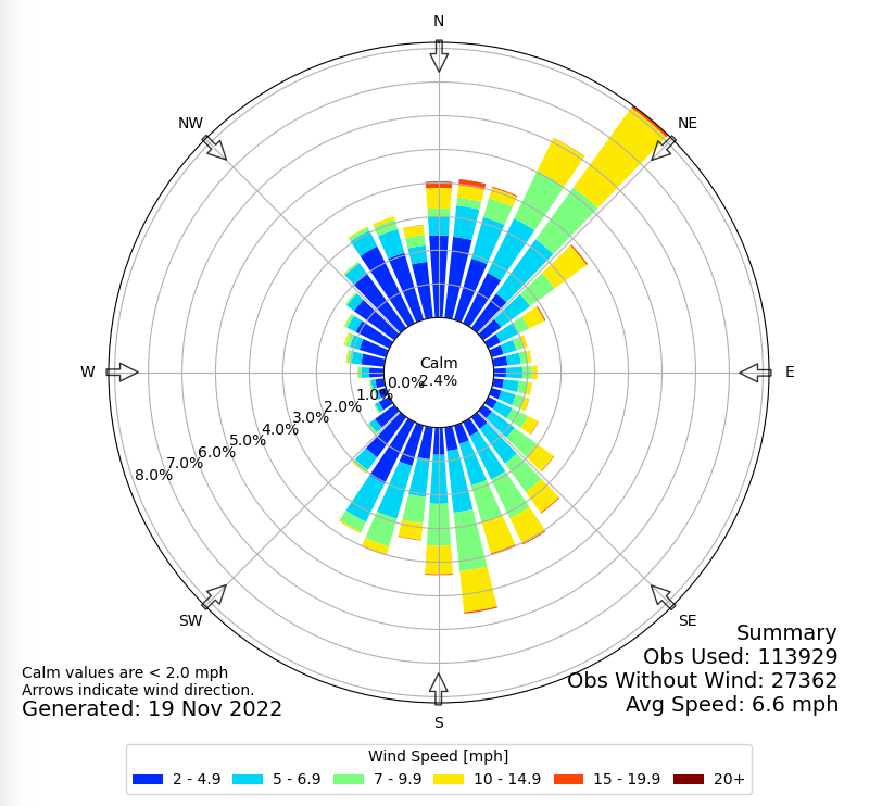
For the safest operations, aircraft take off into the wind, which allows them to lower their takeoff and landing ground speed, and provides additional stability and safety. As a result, the runways for an airport must be oriented in the primary direction of the wind at the site. Figure 5.17 shows a wind rose for the Provo Municipal Airport (PVU); the wind rose shows the percent of the time that wind of a particular strength blows from a particular direction. FAA requires that airports provide runways that can serve the “critical aircraft” 95% of the time. A small general aviation airport may therefore require more crosswind runways than a major international hub, because smaller aircraft have a lower allowable crosswind component, as seen in FAA Table B-1 Figure 5.18.
Note 5.2: The Windy City
Chicago’s O’Hare Airport (ORD, Class E) has six runways on an East-West orientation (270\(^{\circ}\)-90\(^{\circ}\)), and two cross-wind runways on the 220\(^{\circ}\) - 40\(^{\circ}\) azimuth. When the cross-wind component on the main runways is greater than 15 miles per hour, ORD switches to using its cross-wind runways. How often does this happen? A wind rose for ORD is presented below, and full data is in the table following. Assume for this exercise that “greater than 20 mph” means “25 mph” and “15 to 19” means “19”, etc.
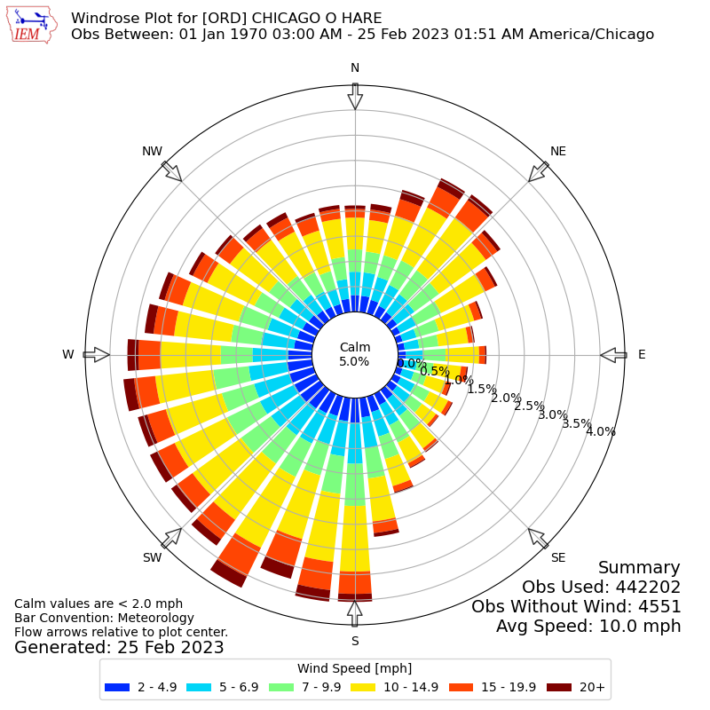
Because the main runways are oriented along the 90\(^{\circ}\) - 270\(^{\circ}\) line, winds blowing from the southwest with an azimuth of 230\(^{\circ}\) are blowing from \(270-230 = 40^{\circ}\) relative to the runway. A wind of 25 mph from this direction has a crosswind component of
\[\begin{align*} &= 25 * \sin((270-230) * \pi / 180)\\ &= 16.1 \mathrm{mph} \end{align*}\]
Because this cross-wind component is greater than 15 miles per hour, aircraft would have to use the cross-wind runways. Repeating for all directions and for the 19 mile-per-hour winds gives the table below.
| Wind direction (0 = N) | Orientation to Runways | % 15-19.9 mph | Component of 19 mph | Crosswind over 15 mph | % > 20 mph | Component of 25 mph | Crosswind over 15 mph | % Crosswind over 15 mph |
|---|---|---|---|---|---|---|---|---|
| 0 | 90 | 0.17 | 19.00 | TRUE | 0.07 | 25.00 | TRUE | 0.24 |
| 10 | 80 | 0.21 | 18.71 | TRUE | 0.12 | 24.62 | TRUE | 0.32 |
| 20 | 70 | 0.34 | 17.85 | TRUE | 0.19 | 23.49 | TRUE | 0.53 |
| 30 | 60 | 0.46 | 16.45 | TRUE | 0.19 | 21.65 | TRUE | 0.65 |
| 40 | 50 | 0.42 | 14.55 | FALSE | 0.14 | 19.15 | TRUE | 0.14 |
| 50 | 40 | 0.28 | 12.21 | FALSE | 0.08 | 16.07 | TRUE | 0.08 |
| 60 | 30 | 0.21 | 9.50 | FALSE | 0.06 | 12.50 | FALSE | 0.00 |
| 70 | 20 | 0.14 | 6.50 | FALSE | 0.04 | 8.55 | FALSE | 0.00 |
| 80 | 10 | 0.10 | 3.30 | FALSE | 0.02 | 4.34 | FALSE | 0.00 |
| 90 | 0 | 0.12 | 0.00 | FALSE | 0.03 | 0.00 | FALSE | 0.00 |
| 100 | -10 | 0.11 | 3.30 | FALSE | 0.03 | 4.34 | FALSE | 0.00 |
| 110 | -20 | 0.08 | 6.50 | FALSE | 0.03 | 8.55 | FALSE | 0.00 |
| 120 | -30 | 0.08 | 9.50 | FALSE | 0.02 | 12.50 | FALSE | 0.00 |
| 130 | -40 | 0.06 | 12.21 | FALSE | 0.01 | 16.07 | TRUE | 0.01 |
| 140 | -50 | 0.08 | 14.55 | FALSE | 0.02 | 19.15 | TRUE | 0.02 |
| 150 | -60 | 0.09 | 16.45 | TRUE | 0.02 | 21.65 | TRUE | 0.11 |
| 160 | -70 | 0.12 | 17.85 | TRUE | 0.03 | 23.49 | TRUE | 0.15 |
| 170 | -80 | 0.23 | 18.71 | TRUE | 0.08 | 24.62 | TRUE | 0.31 |
| 180 | -90 | 0.44 | 19.00 | TRUE | 0.16 | 25.00 | TRUE | 0.60 |
| 190 | -100 | 0.56 | 18.71 | TRUE | 0.23 | 24.62 | TRUE | 0.79 |
| 200 | -110 | 0.57 | 17.85 | TRUE | 0.25 | 23.49 | TRUE | 0.82 |
| 210 | -120 | 0.64 | 16.45 | TRUE | 0.25 | 21.65 | TRUE | 0.88 |
| 220 | -130 | 0.47 | 14.55 | FALSE | 0.16 | 19.15 | TRUE | 0.16 |
| 230 | -140 | 0.39 | 12.21 | FALSE | 0.13 | 16.07 | TRUE | 0.13 |
| 240 | -150 | 0.37 | 9.50 | FALSE | 0.17 | 12.50 | FALSE | 0.00 |
| 250 | -160 | 0.38 | 6.50 | FALSE | 0.20 | 8.55 | FALSE | 0.00 |
| 260 | -170 | 0.42 | 3.30 | FALSE | 0.21 | 4.34 | FALSE | 0.00 |
| 270 | -180 | 0.44 | 0.00 | FALSE | 0.22 | 0.00 | FALSE | 0.00 |
| 280 | -190 | 0.41 | 3.30 | FALSE | 0.18 | 4.34 | FALSE | 0.00 |
| 290 | -200 | 0.37 | 6.50 | FALSE | 0.12 | 8.55 | FALSE | 0.00 |
| 300 | -210 | 0.32 | 9.50 | FALSE | 0.09 | 12.50 | FALSE | 0.00 |
| 310 | -220 | 0.29 | 12.21 | FALSE | 0.08 | 16.07 | TRUE | 0.08 |
| 320 | -230 | 0.29 | 14.55 | FALSE | 0.09 | 19.15 | TRUE | 0.09 |
| 330 | -240 | 0.31 | 16.45 | TRUE | 0.12 | 21.65 | TRUE | 0.43 |
| 340 | -250 | 0.28 | 17.85 | TRUE | 0.09 | 23.49 | TRUE | 0.36 |
| 350 | -260 | 0.20 | 18.71 | TRUE | 0.08 | 24.62 | TRUE | 0.27 |
| Total | NA | NA | NA | NA | NA | NA | NA | 7.18 |
Based on these calculations, ORD will need to use its cross-wind runways approximately 7% of the time. Given that ORD has only 1/3 of its capacity during these periods, it can lead to substantial passenger delay throughout the country.
Runways are numbered with the first two digits of the azimuth of takeoff. So if PVU has its predominant winds blowing from an azimuth of 310\(^{\circ}\), the primary runway will be numbered 31, because planes using that runway will be oriented in that direction. The same runway in the other direction will be labeled 13 because it is pointed at 130\(^{\circ}\). If Provo were to create a second parallel runway in the same orientation, they would be named 31R/13L and 31L/13R for left and right.
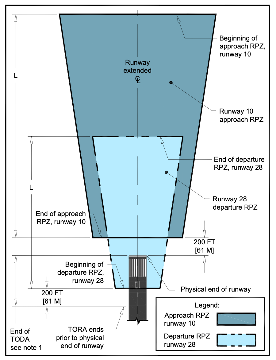
Aircraft must be able to climb on takeoff and descend on approach at a rate that is comfortable for the passengers and safe for the aircraft, as well as protecting property and individuals on the ground. The rate of climb is a function of aircraft weight, speed, runway elevation, and temperature. This means that on hot days, aircraft may not have as much lift and sometimes need to fly at less than their full passenger capacity. Regardless, engineers need to ensure that runways are clear of obstruction for several miles around the airport. This is done with runway protection zones which extend beyond the runway for up to half a mile and must be controlled by the airport or partnering agencies (like a DOT) so that development can be controlled. No buildings or utilities should be put in the RPZ, but roads and some vegetation might be allowed. Figure 5.19 shows the runway protection zones around a small airport in Idaho.
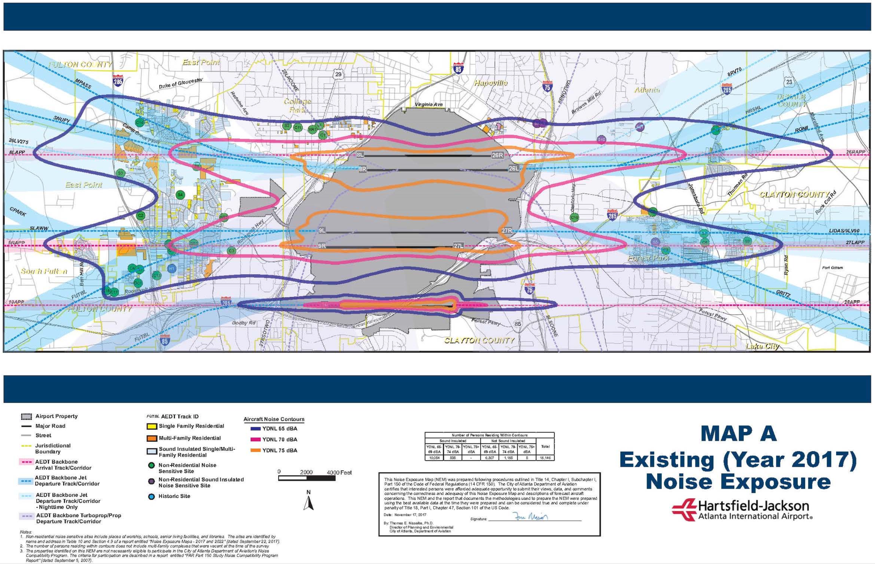
Further beyond the immediate runway protection zone, airliners generate large amounts of noise. This noise is loud enough that it can be harmful to humans exposed to it for long periods. Airports must survey their noise levels and publish noise contours showing the day-night average sound level (DNL). The noise contours for Atlanta’s airport are shown in Figure 5.20. FAA regards a DNL over 60 dBA as inappropriate for residential land uses.
Homework
HW 5.1: Transit Systems
Create a table characterizing the transit systems listed below according to the typology described in the text (ROW, system technology, etc.). What additional transit service might benefit Provo? What characteristics would it have that would be different from the existing services? Include this new service in your table.
- The Ryde campus shuttles
- UTA local buses
- The UVX bus rapid transit system.
HW 5.2: Fuel Efficiency
Find the passenger capacity and average fuel efficiency of a transit bus (in equivalent miles per gallon of gasoline), a recent model year hybrid-electric compact sedan (i.e., Toyota Prius), and a large truck-based family SUV or crossover (i.e., Chevrolet Tahoe) driving in city traffic. Calculate how many people would need to be in the bus for the bus to exceed the per-passenger fuel efficiency of the hybrid sedan and the SUV assuming each car carries only one passenger. How much does this number change if the hybrid and SUV are carrying their full passenger load? What does this show you about fuel efficiency in transportation? Include sources for your fuel efficiency estimates.
HW 5.3: Transit Space Efficiency
Answer the following:
- A freeway lane can carry approximately 2,000 vehicles per hour, and the average passenger occupancy is 1.05 passengers per vehicle. I-15 in Utah County is 5 lanes wide on average. What is the hourly person capacity of I-15?
- A single FrontRunner car can carry 160 people, and the platforms are designed for 10-car trains. A recent proposal in the state legislature would allow for 4 FrontRunner trains per hour. If FrontRunner were running at its full capacity, how many person-equivalent lanes of I-15 would this represent?
- One rail line is approximately 20 ft wide (including envelope), and five freeway lanes is approximately 120 ft wide (including shoulder and roadside).
Which mode is more efficient in terms of space?
HW 5.4: Transit Design
You need to design a peak-period bus network for Provo and Orem. There are three hours in the morning peak, and three hours in the evening peak (6 total hours). A local bus costs \$6.50 to operate per revenue mile, and must have a peak headway of at most 15 minutes. A BRT system costs \$8 per revenue mile and must have a headway of at most 8 minutes. Ignore capital costs, like building the BRT lines and buying vehicles. You have a budget of \$50,000 per day (which must include the costs to operate UVX).
- Print out a scale map of the street network in Provo and Orem (or, you may use a GIS system). Measure the path of UVX to estimate its route length. If UVX runs 6 times per hour during the peak periods, how many peak period revenue miles does UVX consume? How much does it cost to operate during the daily peaks?
- Design a transit route system for Provo and Orem that remains under the daily peak period operating budget. Keep UVX in the design. Your system must serve Intermountain Utah Valley Hospital and downtown [sic] Orem. You should consider other transit trip generators as well, and connections to UVX and FrontRunner. There is a new Vineyard FrontRunner station by 800 North in Orem, which you could include in your plans. You may use a mix of new BRT and new bus service. Provide a map of your system, an estimate of the revenue miles and operating costs, and what design elements you considered when designing your system.
HW 5.5: FrontRunner Regimes
UTA is making plans to extend FrontRunner from Provo to Santaquin. FrontRunner trains have a top speed limit of 79 miles per hour, with an acceleration rate of 2.68 mph/s, a service (non-emergency) braking rate of 2.9 mph/s and a coasting deceleration of \(0.2\) mph/s. The minimum speed allowed during coasting is 65 mph.
The stretch between the Spanish Fork and Payson stations is 6.49 miles. Consider the following possible service designs:
- The vehicle remains at its top speed until braking.
- The vehicle remains at its top speed until it coasts to the point where it begins to brake.
- The vehicle reaches its top speed, coasts to the minimum coasting speed, and re-accelerates until it hits its top speed again. Note: use a whole number of reacceleration periods; figure out how many coast-reaccelerate cycles you can fit in, and maintain your top speed until you start to coast.
- For each scenario, present a time-speed diagram and identify the time at which the train arrives at the next stop.
HW 5.6: FrontRunner Efficiency
Assume that accelerating a FrontRunner train takes 10 units of energy per second, maintaining a speed requires 1 unit of energy per second, and coasting and braking are both 0 units of energy. Calculate the energy used for each of the three service plans in the previous question. Which one is most energy-efficient?
HW 5.7: The delay from stopping a high-speed train
A high-speed rail line is proposed to connect two large cities 200 miles apart. The “constant speed” is expected to be 110 mph, with acceleration and deceleration rates of 3 ft/sec/sec.
- How much time and distance are spent in the acceleration and deceleration phases of the trip between the large cities?
- What if an intermediate stop at a smaller city is added near the halfway point of the trip? If the dwell time at the smaller city is 2 minutes, how much time will be added to the total trip time between the large cities?
HW 5.8: Choosing The Right Freight Mode
| Item | Value [USD] | Weight [lbs] | Rate [USD/ton] |
|---|---|---|---|
| Tulip bulbs | 0.6 | 8.8e-02 | 2400 |
| LED TV | 1500.0 | 5.0e+01 | 4000 |
| Coal [ton] | 20.0 | 2.0e+03 | 10 |
The table above shows the weight, value, and typical shipping rates for several goods.
- Compute the value of a ton of each good.
- The shipping rates for an unspecified freight mode \(X\) is $1000 per ton, regardless of the cargo. Why might a shipper choose to remain with their existing mode instead of switching to mode \(X\)?
HW 5.9: Inventory and Transportation Costs
A piano from a manufacturer in rural Indiana costs $5,000.00, weighs 800 pounds with packing, and is packaged in a custom container 72 inches wide, 54 inches tall, and 27 inches deep. The pianos should not be stacked or rotated vertically.
The trucks available to ship the pianos have a back box 8’ wide, 8’ tall, and 14’ long. The trucks have an empty weight of 10,000 pounds, and a bridge near the factory has a weight limit of 30,000 pounds per truck.
- How many pianos fit into the truck?
- Will the trailer weigh out before it cubes out?
HW 5.10: Freight Analysis Framework
The Freight Analysis Framework (FAF) is a statistical model output created for the Federal Highway Administration (FHWA) by staff at Oak Ridge National Laboratory. The model is estimated from data collected in the Commodity Flow Survey and the 5-year economic census. The most recent update was from data collected in 2024, and was released as an update to FAF5. This product includes a forecast of future freight flows.
Go to the data tabulation tool for the FAF at the Oak Ridge National Laboratory website, and view the “Data Tabulation Tool” Select freight flows originating in Utah (Origin 491 - Salt Lake City and 499 - Rest of UT), and answer the following questions:
- How many total kilotons of freight did Utah produce in the 2022 FAF model?
Now, go find the state-level summary statistics tables, and answer the following questions:
- What percent of that freight (by weight) remained in Utah?
- What state received the largest amount of Utah’s domestic exports (by weight)?
- Of the freight leaving Utah and going to other US States (not exported internationally), what is the mode share by weight? That is, what percent of freight leaving Utah goes by truck versus pipeline versus air?
- Of the freight leaving Utah and going to other US States (not exported internationally), what is the mode share by value? (Find the sheet in the excel workbook labeled “Value”)
- What are the top three commodities shipped to Utah from other states by weight?
- What are the top three commodities shipped to Utah from other states by value?
HW 5.11: Aviation Data
Search the World Wide Web to get more current values for the items listed below. For each item, provide the most recent value you can find, the year of that value, the source of that information, the search engine you used, and the key words you used to do the search. A.Total number of US airports B.Number of commercial aircraft C.Number of general aviation aircraft D.Miles flown by commercial aircraft E.Passengers carried by commercial aircraft F.Hours flown by general aviation aircraft
HW 5.12: Growth in domestic air travel
Find the current edition of National Transportation Statistics.
A. Cite the URL for the NTS edition you use. In what year was it published? In what table did you find data on the number of passenger enplanements?
B. What are the first and last years in the table? How many enplanements took place in those years? C. What is the average percent change per year in passenger enplanements, from the earliest year to the most recent year in the table?
HW 5.13: Measuring airport delay
Use the most recent version of the Bureau of Transportation Statistics website on airport delay.
- What was the percent on-time arrivals for all US airports in the last full calendar year for which data are available?
- What was the on-time for Salt Lake City International Airport in the last full calendar year for which data are available?
- Find an airport with percent on-time arrivals < 70%. (Hint: Try the New York City area.) What are its two most frequent causes?
HW 5.14: Runway Orientation
The windrose below is for a major airport in Asia that serves only large commercial airliners.
- How many runway orientations are likely needed at this airport?
- Assume that airport capacity requires two parallel runways. What will they be numbered?
- The strongest recorded winds on the rose are from due north. What is the maximum recorded crosswind speed on the main runway?
- Extra credit What is the airport?
HW 5.15: Bike Walk Provo
Bike Walk Provo is an advocacy organization that tries to encourage the Provo City Council to improve the infrastructure for biking and walking in Provo. They have created self-guided bike and walk tours of Provo. Go on one of the tours; you may choose to do the biking or the walking tour. The tours are different, so you could do both! But you only need to do one for this assignment.
Each tour has both a map and a playlist of YouTube videos at each stop. If you can, watch the videos on your phone when you are at each stop of the tour. Otherwise, I would recommend watching the videos before you take the tour. You may also elect to schedule a time with a Bike Walk Provo volunteer.
Turn in a short (less than a page)write-up describing:
- Something you learned about designing for pedestrians / cyclists that you hadn’t thought of before.
- Is there a place in Provo that should be redesigned with a specific infrastructure or facility to improve the safety and ease of walking or biking?
If you are unable to walk or bike for long distances, please contact the instructor for an alternate assignment.
References
Laver, R., Schneck, D., Skorupski, D., Brady, S., & Cham, L. (2007). Useful life of transit buses and vans.
Walker, J. (2012). Human transit: How clearer thinking about public transit can enrich our communities and our lives. Island Press.