
3 Roadway Elements
When engineers actually set out to design roadways, there are a number of considerations they need to take into account. Foremost among these is ensuring that motorists can operate their vehicle safely along the road. This sometimes requires that engineers reshape the earth to make hills and valleys longer. It also requires that drivers are constantly informed of upcoming roadway conditions. In this unit, you will learn how to:
- Use the dynamic interaction of the driver, roadway, and vehicle, to evaluate and design roadway sections for safe stopping sight distance.
- Determine key dimensions of horizontal and vertical alignments of roadway sections using safe stopping sight distance and superelevation.
- Determine when an intersection warrants the installation of a traffic signal, design signal settings for intersections so that drivers will not face a dilemma zone, and understand that congestion and associated delays are societal costs.
3.1 Vehicle and Driver Dynamics
Automobiles and other roadway vehicles are complex machines with capability to accelerate, turn, brake, and generally move down the roadway. The performance of individual vehicles when doing these tasks varies based on the vehicles’ engines, their tires, and the conditions of the roadway surface. At the same time, these vehicles are operated by (usually) amateur motorists who have limited and varied capacity for observing and processing information, and for reacting to stimuli. Engineers need to design roads so that a baseline motorist operating a baseline vehicle can react to turns, stops, and other roadway elements in a safe and controlled manner.
3.1.1 Driver Reactions
When a driver sees something ahead on the road, their brain steps through four distinct processes:
- Perception: The driver sees that there is an object or situation ahead.
- Identification: The driver realizes what the object or situation is.
- Emotion: The driver reacts to the object or situation with a feeling.
- Volition: The driver decides how to react.
Each of these reactions takes time. The total amount of time to go through all four steps is highly variable between situations and people: a Formula 1 driver in a race will react much more quickly than a middle-aged, non-athletic engineering professor driving casually down an urban arterial. But various studies have determined that a total reaction time \(t_r = 2.5\) seconds is an appropriate reaction time for most drivers in typical situations. The distance covered during this time is the reaction distance \(d_r\),
\[ d_r = t_r * v \tag{3.1}\]
where \(v\) is the speed of the vehicle. Note that the units of speed and time may need to be converted to be compatible.
3.1.2 Visual Acuity
In order for a driver to react to instructions provided by the roadway — for instance through direction signs — they need to be able to see them. While some visual ques, such as a deer crossing the road, cannot be controlled, roadway signs and pavement messages can be designed to give the driver ample time to respond. Roadway signs and pavement messages should be designed so that travelers on the road can read them from an appropriate distance. We can use trigonometry to estimate how tall the lettering should be based on a person’s angle of vision for reading.
Using the geometry presented in Figure 3.1, we can derive an equation relating how tall \(H\) the letters on a sign must be to be seen at distance \(D\) \[ \frac{H/2}{D} = \tan{\frac{\theta}{2}} \tag{3.2}\] where \(\theta\) is the angle of visual acuity for reading (in radians), or the angle of the vision field at which people can read effectively. Since most people have a narrow angle of sight for reading (usually about 0.002 radians) and because \(D\) is almost always substantially larger than \(H\) for roadway signs, we can simplify this equation as \[ \frac{H}{D} \approx \theta \tag{3.3}\]
3.1.3 Stopping Sight Distance
Recall from physical dynamics that the energy of a moving object is \[ E = mv^2 / 2 \tag{3.4}\] where \(m\) is the mass of the object, and \(v\) is its speed. The work necessary to bring an object to a rest across a level surface over a distance \(d\) is \[ W = f_r m g d \tag{3.5}\] where \(g\) is the gravitational constant and \(f_r\) is a friction coefficient. Setting Equation 3.4 and Equation 3.5 equal to each other will allow us to solve for the stopping distance \(d\) at that particular amount of energy,
\[\begin{align*} f_r m g d &= mv^2 / 2 \\ d &= \frac{v^2}{2 f_r g} \end{align*}\]
Note 3.1: Mass of vehicle
Note that the mass of the vehicle \(m\) cancels out of this equation, meaning that the size of the vehicle does not affect its stopping distance. Is this intuitive?
Of course, two additional elements are required to understand how far it will take a car to stop. First, we know from the previous section that there will be some amount of reaction time \(t_r\). Also, roads are not always level, so we need to accommodate the grade of the road, \[ SSD = vt_r + \frac{v^2}{2g(f_r \pm G)} \tag{3.6}\] where \(G\) is the grade of the road in the direction of travel; that is, a 4% downhill grade will result in \(G = -0.04\).
The coefficient of rolling friction (\(f_r\)) itself changes based on the initial speed, as well as the particular tires installed on the car. Baseline values estimated by AASHTO for use in design can be obtained from Table 3.1.
| Initial Speed [mph] | Friction coefficient $f_r$ |
|---|---|
| 20 | 0.40 |
| 25 | 0.38 |
| 30 | 0.35 |
| 35 | 0.34 |
| 40 | 0.32 |
| 45 | 0.31 |
| 50 | 0.30 |
| 55 | 0.30 |
| 60 | 0.29 |
| 65 | 0.29 |
| 70 | 0.28 |
Because all the roads we are currently building are on Earth, and because the units of speed, time, and distance are often consistent across problems, we can simplify this equation as \[ SSD = 1.47 V t_r + \frac{V^2}{30(f_r \pm G)} \tag{3.7}\] where SSD is in feet, \(V\) is in miles per hour, \(t_r\) is in seconds and \(V\) is in miles per hour.
Warning 3.1: Units and conversions
Equation 3.6 is the exact version of the stopping sight distance equation that comes from the physical derivation. Equation 3.7 is the version that often appears in the FE exam or design manuals, and contains a number of approximate unit conversions. The two equations give effectively the same answer for practical purposes, but on the assignments and exams in this class you may be asked to give the answer from one equation or the other.
Note that according to kinematics the denominator in the SSD equation \(2g(f_r \pm G)\) is the total deceleration of the vehicle. In some cases the deceleration is given by the problem, meaning that we need to rearrange this as \[ f_r = \frac{a}{g} \tag{3.8}\]
Additionally, Equation 3.6 can be derived not to calculate the distance to stop, but the distance to transition from one speed to another: \[ d_{v_0 v_f} = v_0t_r + \frac{v_0^2 - v_f^2}{2g(f_r \pm G)} \tag{3.9}\]
where \(v_0\) is the initial speed and \(v_f\) is the final speed. The second part of this equation is the distance traveled while braking or accelerating; occasionally we need to calculate the time to change speeds rather than the distance. This can be derived as
\[ t_{v_0 - v_f} = \frac{v_0 - v_f}{g(f_r \pm G)} = \frac{v_0 - v_f}{f_rg} = \frac{v_0 - v_f}{a} \tag{3.10}\]
When designing facilities, engineers will often use values for stopping sight distance that are tabulated for different speeds in the AASHTO A Policy on the Geometric Design of Highways and Streets design manual, which is recreated in Table 3.2.
| Design Speed (mph) | Reaction Distance (ft) | Braking Distance (ft) | Calculated SSD (ft) | Design SSD (ft) |
|---|---|---|---|---|
| Calculated distances are based on a 2.5-second reaction time, level grade, and a deceleration rate of 11.2 ft/s$^2$. | ||||
| 15 | 55 | 22 | 77 | 80 |
| 20 | 73 | 38 | 112 | 115 |
| 25 | 92 | 60 | 152 | 155 |
| 30 | 110 | 86 | 196 | 200 |
| 35 | 128 | 118 | 246 | 250 |
| 40 | 147 | 154 | 300 | 305 |
| 45 | 165 | 194 | 359 | 360 |
| 50 | 183 | 240 | 423 | 425 |
| 55 | 202 | 290 | 492 | 495 |
| 60 | 220 | 346 | 566 | 570 |
| 65 | 238 | 406 | 644 | 645 |
| 70 | 257 | 471 | 727 | 730 |
| 75 | 275 | 540 | 815 | 820 |
| 80 | 293 | 615 | 908 | 910 |
3.2 Roadway Signs and Markings
Safe traffic operations require that drivers know where they are supposed to be, and how and when they are supposed to move. Roadway signs, traffic signals, pavement markings, and other similar indications are considered traffic control devices. Transportation engineers are involved with specifying and desinging traffic control devices, as well as ensuring that they are well-maintained.
The Manual on Uniform Traffic Control Devices (MUTCD) is a mandatory federal regulation that state and local agencies must follow if they are to receive federal transportation funds. The current MUTCD — whose cover is shown in Figure 3.2 — was newly issued in 2023. In coming years, it may be updated with improvements some error corrections.
According to the MUTCD, there are five requirements a traffic control device must meet:
- Fulfill a need — Unnecessary signs and markings confuse drivers and reduce the effectiveness of necessary ones.
- Command attention — Control devices should be installed in such a way that they are unmissable. Drivers should be able to see them clearly.
- Convey a clear, simple meaning — Signs and markings should be unmistakeable: nothing else should look like a stop sign, or a caution sign, etc.
- Command respect from road users — Redundant or confusing signs will be ignored by drivers.
- Be placed to get the proper response from the driver — Navigation signs should be place where people need to make decisions, neither unnecessarily early nor too late.
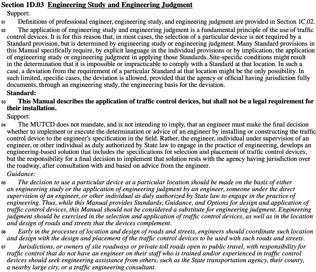
The MUTCD contains varying levels of standards, guidance, and support. The verbs used in the manual are carefully chosen to reflect what engineers shall do, what they should do, and what they may do with respect to traffic control devices. An example of this language is given in Figure 3.3: the Standard described in Section 1A.09 means that the MUTCD describes how traffic control devices shall be installed and used, but that engineering judgment is required to know which devices are necessary or useful. That said, engineers whose “judgment” directly contradicts the standards and guidance in the MUTCD have been found liable in wrongful death lawsuits.
Roadway signs serve a number of purposes: posting the speed limit, alerting drivers to upcoming turns, or identifying route junctions. The MUTCD includes several classifications of signs and markings, with distinctive rules about the colors used, the shapes of the signs, and their placement.1
3.2.1 Regulatory
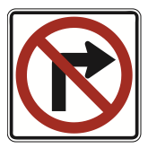
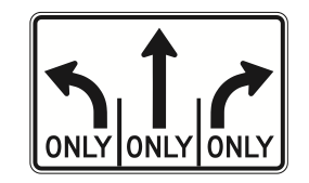
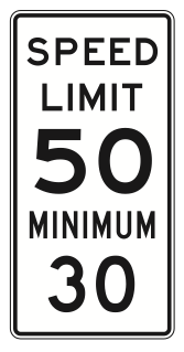
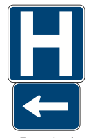
Regulatory signs and markings describe how vehicles shall behave in the traffic stream. Generally, regulatory signs are rectangular with black letters on a white background. Sometimes red may be incorporated in the sign to warn drivers of immediate conflict, as in wrong way, yield, turn restrictions, and stop signs. No other kinds of sign may use red. Example regulatory signs are shown in Figure 3.4.

3.2.2 Warning
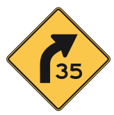
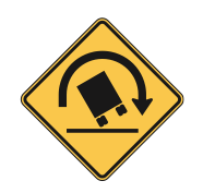
Warning signs and markings alert drivers to unusual or potentially dangerous conditions, including turns, grades, crossings, etc. These signs involve black text on a yellow background, and are either diamond-shaped or rectangular. Example warning signs are shown in Figure 3.5.
3.2.3 Guide
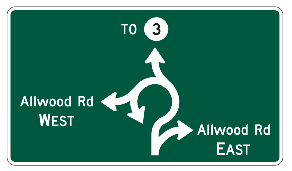
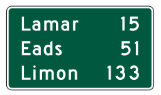
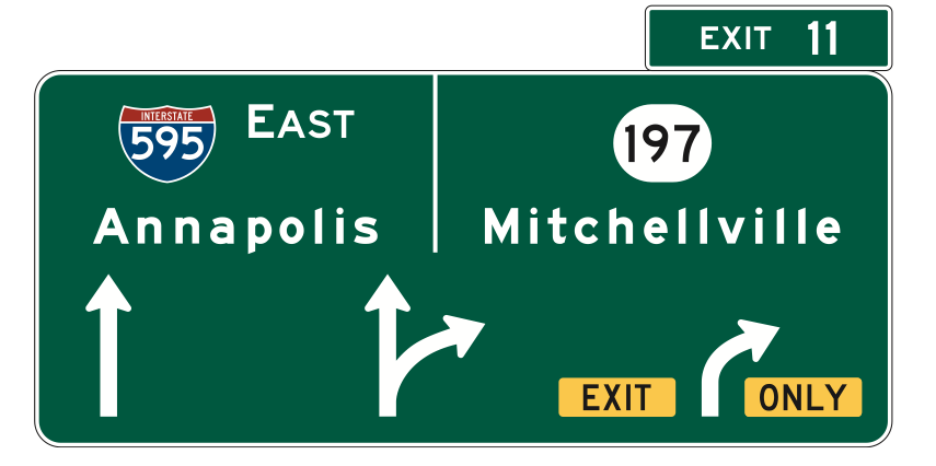
Guide signs instruct drivers on how to navigate on the road system, including directions, upcoming exits, and street signs. These signs usually have white text on a green background. Example guide signs are shown in Figure 3.6.
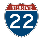
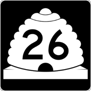
A special category of guide signs that are allowed to diverge from the green background are route markers. Interstates are shown with a blue and red union shield, other federal highways have a white shield, and state routes are often branded with a state emblem, as shown in Figure 3.7.

Beginning with the 2009 MUTCD, toll roads and other managed lanes on general facilities can be indicated with special purple backgrounds, as illustrated in Figure 3.8.
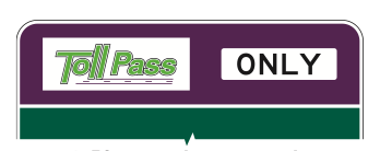
TipThink
The MUTCD reserves two additional colors for signs that it does not currently have an application for: coral (pink) and a light blue. Prior to 2009, purple was a reserved color that now applies to toll lanes. What kind of purposes could you imagine these other reserved colors applying to?
3.2.4 Temporary Control
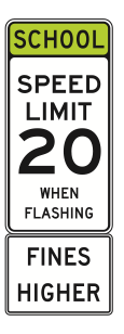
Work zones and other temporary traffic control devices require special attention to alert unfamiliar drivers of particularly risky situations. These signs involve black text on an orange background. The signs themselves are diamond-shaped, but can have additional rectangular notes. Examples are shown in Figure 3.9. Note how elements of these signs that serve another purpose — like the work zone speed limit — are presented in their appropriate regulatory colors, with orange appended to indicate the temporary control nature of the sign.
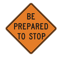
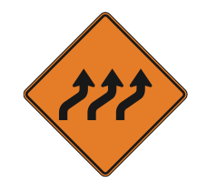
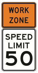
Other temporary traffic control devices — including cones, barrels, and flags — shall also be orange.
3.2.5 General Information
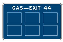
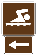
Signs can inform drivers of upcoming destinations and services. Public attractions are shown on brown signs, and services including gas stations, lodging, and hospitals with blue signs. Examples are given in Figure 3.10.
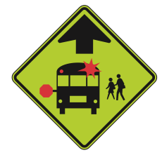
3.2.6 School Zones
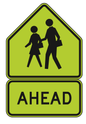
School zones require special markings to reflect that the pedestrians in the area may be especially vulnerable. School zones are designated with black text on a fluorescent yellow-green background and a special “schoolhouse” pentagonal shape. Other school-related signs should also be fluorescent yellow-green, but might be on diamond-shaped caution-style signs as illustrated in Figure 3.11.
3.2.7 Pavement Markings
Pavement markings also use different patterns and colors to inform drivers about the roadway. Occasionally, pavement markings convey messages through text or symbols — e.g. “stop ahead” markings and bicycle lane “sharrows” — but they usually convey messages through lines. Generally, solid lines mean crossing them is discouraged or prohibited, and dashed lines mean it is permitted to cross them. Additionally, line color and and pattern are combined in various ways to indicate more specific information.
- Yellow lines separate traffic going in opposite directions.
- Dashed yellow lines on the travelers’ side indicate permission to pass using the opposing lane when it is safe to do so.
- Solid double yellow lines indicate that crossing them is prohibited.
- Single solid yellow lines indicate the left inside edge of a divided roadway.
- White markings separate traffic going in the same direction.
- Dashed white lines indicate that lane changing is permitted.
- Solid white lines strongly discourage crossing them. (These can be used in several ways such as separating certain lanes from the rest of traffic, or marking the outside edge of a pavement or shoulder.)
The 2023 MUTCD includes new pavement markings that are already in use in some jurisdictions:
- Bike lanes that are separated from or shared with vehicle lanes may be painted green.
- Americans with Disabilities Act (ADA) reserved parking spaces may be painted blue.
- Bus-only lanes may be painted red.
- Toll plaza approach lanes restricted to use by vehicles with electronic toll collection may be painted purple
3.3 Highway Alignment
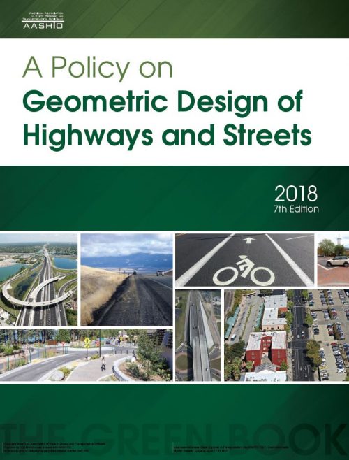
Engineers must design highways to fit the geometry of the terrain while meeting certain design standards. This practice is commonly called Geometric Design. AASHTO has published a thorough documentation of geometric design standards called A Policy on Geometric Design of Highways and Streets, or more colloquially, The Green Book. These standards may be supplemented by policies set forth by state DOTs, but we will focus on The Green Book standards in this section. The primary goals of effective geometric design are as follows:
- Roadways designed on hills and curves should allow drivers to see and avoid obstacles ahead.
- Proposed highway sections are defined according to stationing conventions.
- Roadway realignments around specific locations, (e.g. protected wetlands,) must be well justified.
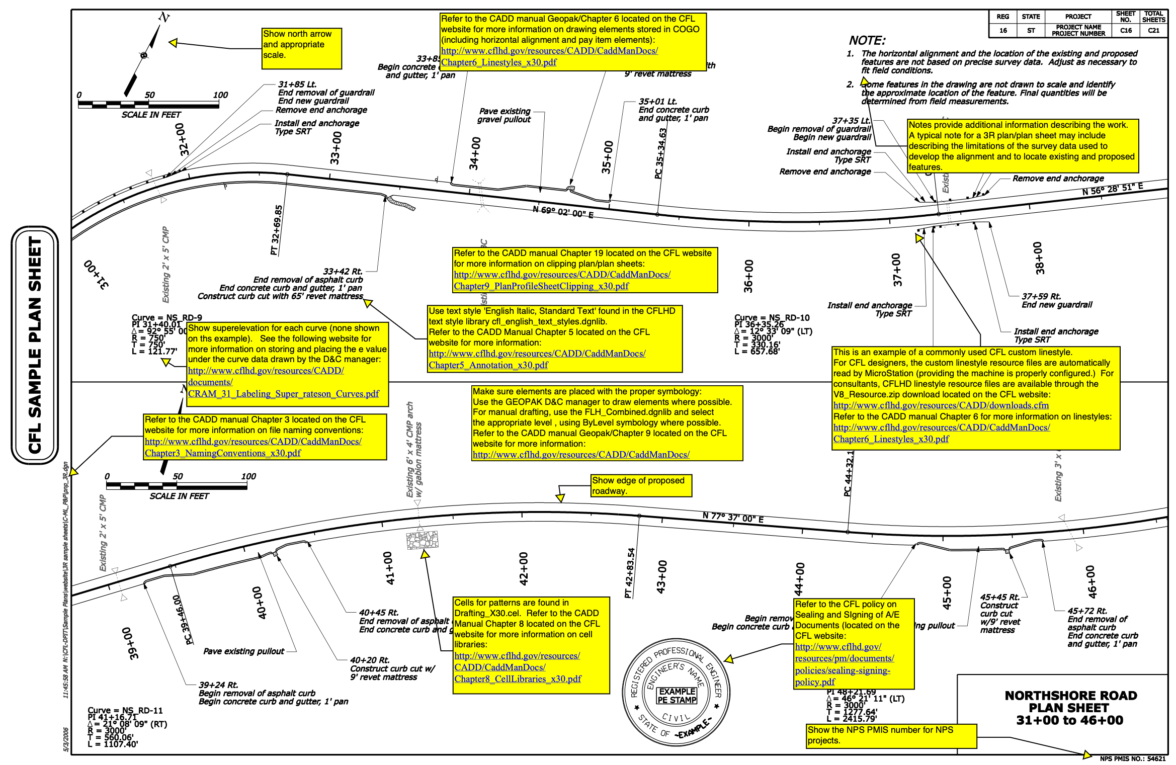
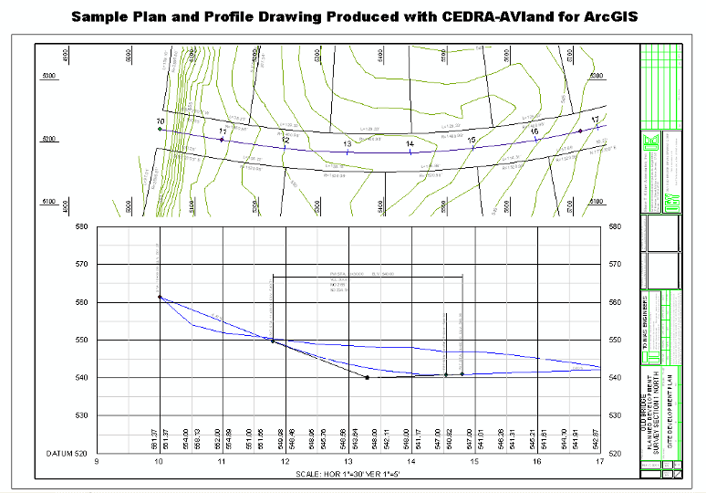
- The design drawings for roadways follow specific standards.
3.3.1 Stationing
When engineers survey, design, and construct a roadway, a convention called stationing is used to determine where the road elements are. Each station is 100 feet long, and is measured along the centerline of the roadway. So a point that is 2,410.8 feet from a reference point will have station \(24 + 10.8\).
Stationing is always level in the plane. That is, when you look at a road in profile, the stationing will proceed along the \(x\)-axis regardless of how the road is curved, as shown in Figure 3.13.

It may seem strange for stationing not to follow the surface of the road. But this is important when considering the horizontal layout of a roadway; engineers reading plan sheets should not need to take into account the slope of the road when measuring distances on those sheets. Stationing for horizontal curves follows the centerline of the roadway, as shown in Figure 3.14.
3.3.2 Vertical Curves
Vertical Curves in roadway design occur whenever there is a change in Grade (slope) along a section of the road. Curves that concave up are referred to as Sag Vertical Curves while curves that concave down are referred to as Crest Vertical Curves. Figure 3.16 depicts these different types of vertical curves. Vertical are designed as parabolas.
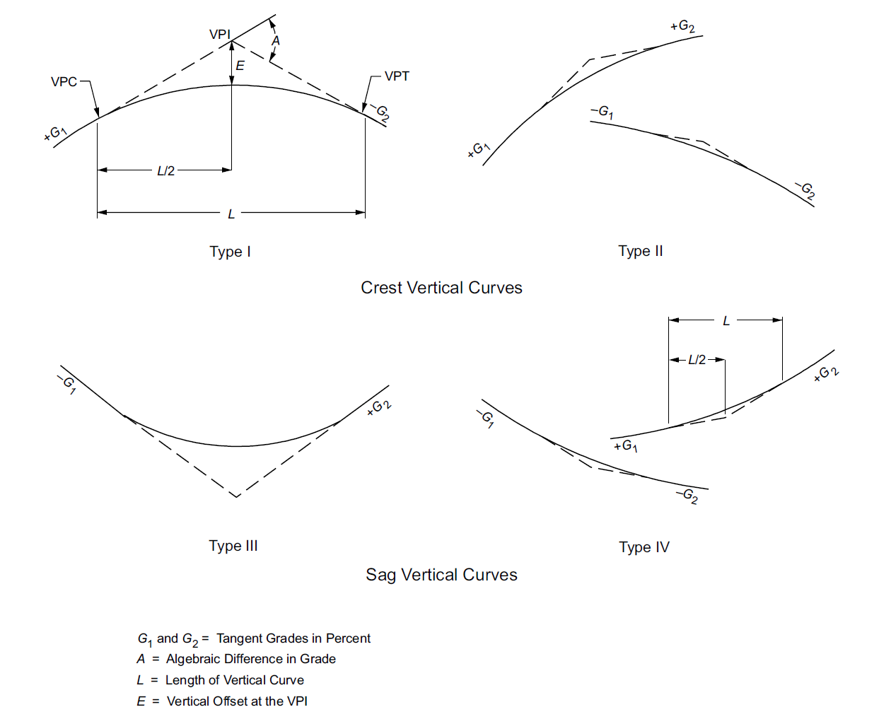
TipVertical Curve Types
Note that one way to determine whether a curve is a crest vertical curve is when \(G_1 > G_2\). Likewise, sag vertical curves occur when \(G_1<G_2\).
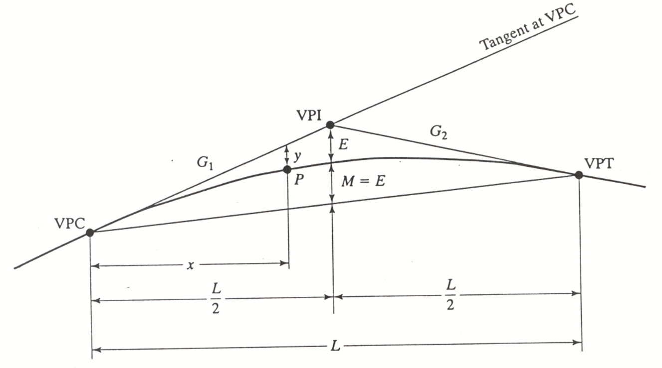
The geometric elements of a vertical curve are shown in Figure 3.17 and are described as:
- \(G_1\) and \(G_2\): the incoming and outgoing grades, which will usually be given in percents (e.g. 4%), but algebraically are used as decimals.
- \(VPC\): The point where the curve begins is called the Vertical Point of Curvature.
- \(VPT\): The point where the curve ends and returns to a constant grade is called the Vertical Point of Tangency.
- \(L\): The total length of the curve, measured horizontally between the \(VPC\) and \(VPT\)
- \(VPI\): The point where the tangents created by both grades intersect is called the Vertical Point of Intersection. Because these curves are asserted to be equal tangent curves, \(VPI = L/2\).
- \(x\): The horizontal coordinate of a point the curve, measured horizontally from the \(VPC\).
- \(Y\): The vertical coordinate of a point on the roadway surface
- \(\gamma\): the vertical offset from the first tangent to the surface of the roadway (for equal-tangent curves).
Starting from the basic equation for a parabola, \[ Y = a + bx + cx^2 \tag{3.11}\] we need to derive values for \(a\), \(b\), and \(c\) in terms of the curve geometry. The intercept of the curve \(a\) is simply the elevation of the \(VPC\). \[ a = Y(VPC) \tag{3.12}\] The derivative of the parabola with respect to \(x\) \(dy/dx\) is the grade at each point. Because we know the grade at each end of the curve, we can solve for the \(b\) and \(c\) parameters: \[\begin{align*} \frac{dy}{dx} = Y'(x) &= b + 2cx\\ Y'(0)&= G_1 = b + 2c (0)\\ b &= G_1 \\ Y'(L)&= G_2 = G_1 + 2c (L)\\ \end{align*}\] \[ c = \frac{G_2-G_1}{2L} \tag{3.13}\] So to be complete, \[ Y = Y(VPC) + G_1x + \frac{G_2 - G_1}{2L}x^2 \tag{3.14}\]
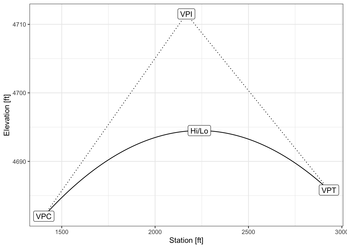
The point \(x\) at which \(\frac{dy}{dx}=0\) is either the high or the low point of the curve: \[ Y'(x_{hi/lo})= 0 = G_1 + \frac{G_2-G_1}{2L}x_{hi/lo}\\ \] \[ x_{hi/lo} = L \times \frac{G_1}{G_1-G_2} \tag{3.15}\]
Warning 3.2: Vertical curve high/low point
It is a common misconception to believe that the high or low point on a curve occurs at the same place as the VPI. Remember that the VPI is the location where the incoming and outgoing grades intersect, and not the high or low point on the curve. This is most evident in Type II and Type IV curves as depicted in Figure 3.16. In fact, notice that the high or low point occurs at either the VPC or VPT for Type II and Type IV curves. When this is the case, Equation 3.15 will not be effective for determining the high or low point on the curve.
Another important consideration is the offset \(\gamma\) between the line of tangency and the actual roadway curve. The tangent line is simply \(Y_T = Y(VPC) + G_1x\), meaning that the offset can be derived as \[\begin{align*} \gamma&=Y(x) - Y_T\\ &=\left[Y(VPC) + G_1x + \frac{G_2 - G_1}{2L}x^2\right] - \left[Y(VPC) + G_1x\right]\\ \end{align*}\] \[ \gamma = \frac{G_2 - G_1}{2L}x^2 \tag{3.16}\]
A key value used in roadway design is the degree of curvature \(K\)2: \[ K = L / A \tag{3.17}\] Where \(A\) is the absolute difference in grades as percentages.
3.3.2.1 Crest Vertical Curves Design Length
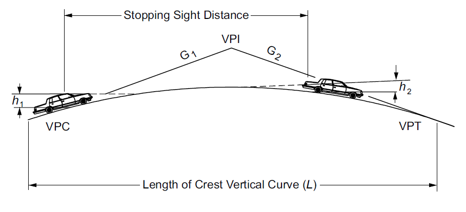
On a crest vertical curve, engineers must design the road so that drivers can always see far enough ahead to stop for an object in the road, as shown in Figure 3.18. The derivation of this is tricky, and changes based on whether the object is on the curve or lies on the tangent on the other side of the curve. As a result, we have two equations:
\[ L_{min1} = \frac{|A|\cdot S^2}{100(\sqrt{2h_1}+\sqrt{2h_2})^2} \; \mathrm{for} \, S\leq L \tag{3.18}\]
\[ L_{min2} = 2S - \frac{200(\sqrt{h_1}+\sqrt{h_2})^2}{|A|} \; \mathrm{for} \, S> L \tag{3.19}\]
In both equations:
- \(A\) is the algebraic difference in the percent grades3,
- \(h_1\) is the assumed height of the driver’s eye, usually 3.5 feet.
- \(h_2\) is the assumed height of an object that must be avoided, usually assumed to be 2 feet tall.
It is not generally possible to determine which minimum distance will govern, so you must calculate both equations and choose the one that applies. You may choose a stopping sight distance based on the applicable design speed from Table 3.2, if the assumptions of 2.5 second reaction time and 11.2 \(\mathrm{ft}/\mathrm{sec}^2\) apply to your situation.
3.3.2.2 Sag Vertical Curve Design Length
During daytime, drivers on a sag vertical curve can see the entire curve, and stopping sight distance is not a concern. But at night, drivers can only see as far ahead as their headlights can illuminate the road ahead. Figure 3.19 shows how to design a sag vertical curve for SSD based on the height and angle of the headlights. The minimum acceptable length for the vertical curve is determined from these parameters.
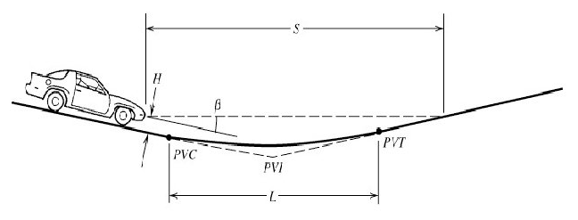
If a car has headlights at height \(h\) (usually 2 feet) and an effective illumination angle of \(\beta\) (usually \(1^{\circ}\)), the minimum length of the curve is either
\[ L_{min1} = \frac{|A|\cdot S^2}{200(h+S\tan(\beta))} \; \mathrm{for} \, S\leq L \tag{3.20}\] \[ L_{min2} = 2S - \frac{200(h+S\tan(\beta))}{|A|} \; \mathrm{for} \ S>L \tag{3.21}\]
Again, you may choose a stopping sight distance based on the applicable design speed from Table 3.2 if the assumptions of the table can apply.
3.3.2.3 K Factors for vertical curves
Rather than designing the minimum allowable vertical curve length, we can also design for the maximum allowable rate of vertical curvature, \(K\).
Table 3.3 shows design K factors for sag and vertical curves based on design speed and SSD.
| Rate of Vertical Curvature $K$ | |||
|---|---|---|---|
| Design Speed (mph) | Design SSD (ft) | Crest Curves | Sag Curves |
| Calculated distances are based on a 2.5-second reaction time, and a deceleration rate of 11.2 ft/s$^2$. | |||
| 15 | 80 | 3 | 10 |
| 20 | 115 | 7 | 17 |
| 25 | 155 | 12 | 26 |
| 30 | 200 | 19 | 37 |
| 35 | 250 | 29 | 49 |
| 40 | 305 | 44 | 64 |
| 45 | 360 | 61 | 79 |
| 50 | 425 | 84 | 96 |
| 55 | 495 | 114 | 115 |
| 60 | 570 | 151 | 136 |
| 65 | 645 | 193 | 157 |
| 70 | 730 | 247 | 181 |
| 75 | 820 | 312 | 206 |
| 80 | 910 | 384 | 231 |
3.3.3 Horizontal Curves
Horizontal Curves occur whenever the roadway changes direction laterally. Horizontal curves are designed as arcs, meaning they follow a circular path. The elements of horizontal curves are shown in Figure 3.20. The beginning of the curve is called the Point of Curvature (PC), and the end of the curve is called the Point of Tangency (PT). The point where the tangent line to the PC and the tangent line to the PT intersect is called the Point of Intersection (PI). Unlike vertical curves, the length (L) of the horizontal curve is measured along centerline of the curve from the PC to the PT.
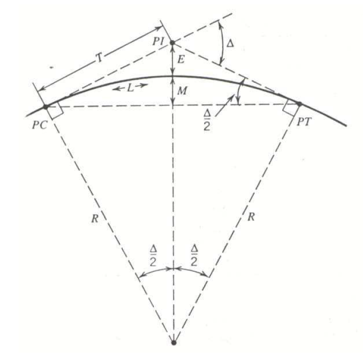
The elements of horizontal curves are:
- \(PC\) = Point of Curvature (start of horizontal curve)
- \(PT\) = Point of Tangency (end of horizontal curve)
- \(PI\) = Point of (tangent) Intersection
- \(L\) = length of horizontal curve
- \(D\) = Degree of curvature (\(^{\circ}\) per 100 ft of centerline)
- \(R\) = Radius of the curve (measured to centerline)
- \(\Delta\) = Central angle of curve in degrees
- \(T\) = Tangent length
- \(M\) = Middle ordinate
- \(LC\) = Length of long chord (straight line from \(PC\) to \(PT\))
- \(E\) = External distance
3.3.3.1 Horizontal curve equations
Since horizontal curves are designed as circular arcs, calculating the elements for them is relatively straightforward. Equation 3.22 through Equation 3.27 may be used for calculating these elements. The Degree of Curvature (D) is the degrees that the curve deflects for every 100 feet along the curve,
\[ D = \frac{100 * (180 / \pi)}{R} = \frac{5729.6}{R} \tag{3.22}\]
\[ L = \frac{100\Delta}{D} \tag{3.23}\]
\[ T = R\tan(\frac{\Delta}{2}) \tag{3.24}\]
\[ M = R(1-\cos(\frac{\Delta}{2})) \tag{3.25}\]
\[ LC = 2R\sin(\frac{\Delta}{2}) \tag{3.26}\]
\[ E = R\left(\frac{1}{\cos(\frac{\Delta}{2})}-1\right) \tag{3.27}\]
3.3.3.2 Stationing along horizontal curves
Just like with vertical curves, horizontal curves are measured in stations. The PC does not always begin at the origin, so distances relative to the PC may need to be converted to stations by adding the station of the PC. For horizontal curves, stations are measured along the length of the horizontal curve, meaning they are measured along the curve itself, not in a straight line.
3.3.3.3 Horizontal curve design for sight distance
Figure 3.21 shows how to design a horizontal curve for stopping sight distance (SSD) based on the distance from the roadway to a sight obstruction. This distance is known as the Horizontal sight line offset (HSO). Note: in the past, the HSO was called the Middle Ordinate (\(M_s\)) so either term is acceptable. If the HSO is too small, the sight obstruction may need to be cut back or the road built further away. It is important to know that the HSO is measured from the sight obstruction to the middle of the inside lane, not the centerline.
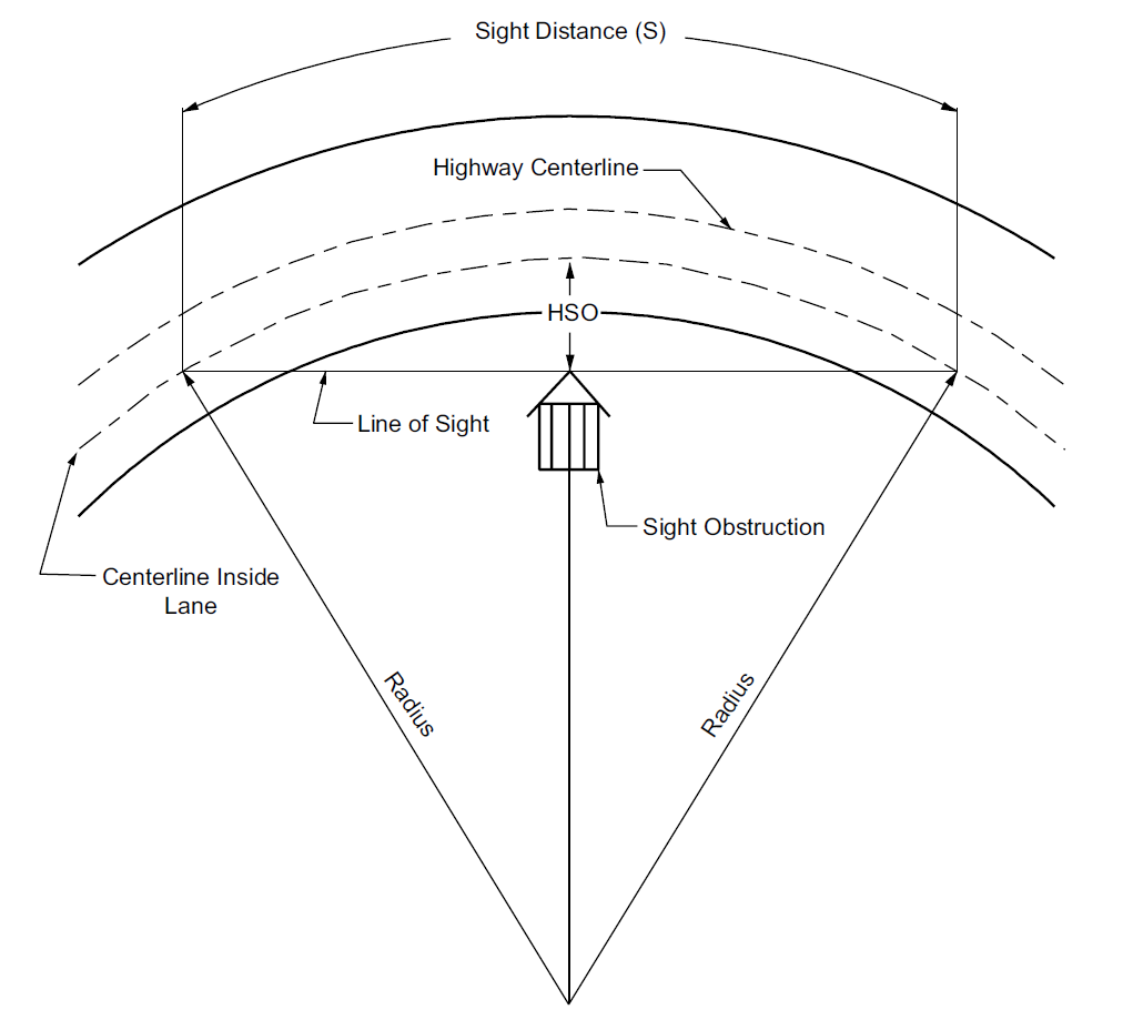
Equation 3.28 may be used to calculate the minimum acceptable distance for the HSO or \(M_s\). This is necessary if we are not willing to change the design SSD by lowering the design speed.
\[ M_s = R_v\left(1-\cos(\frac{\Delta_s}{2})\right) = R_v\left[1-\cos\left(\frac{90\times SSD}{R_v\pi}\right)\right] \tag{3.28}\]
where:
- \(M_s\) = Middle ordinate (or Horizontal sight line offset)
- \(R_v\) = Radius of the curve (measured to the middle of the inside lane)
- \(\Delta_s\) = Angle of the portion of the curve that is as long as the SSD
- \(SSD\) = Stopping sight distance
Warning
Notice that the length of the horizontal curve needs to be at least as long as the SSD for Equation 3.28 to be valid. Cases where the curve is not as long as the SSD are not covered in this section.
Alternatively, we may need to set the design speed based on the existing SSD if the sight obstruction is permanent and can’t be moved. In this case, we can calculate the SSD from Equation 3.29.
\[ SSD = \frac{R_v\pi}{90}(cos^{-1}(\frac{R_v-M_s}{R_v})) \tag{3.29}\]
3.3.3.4 Superelevation
Due to the forces involved in going around a horizontal curve, drivers may feel uncomfortable or their tires might even slip while traveling around a horizontal curve if the roadway is flat. This issue is mitigated by banking the roadway. We measure banking by the superelevation rate (e). The goal of superelevation is not necessarily to eliminate the lateral force on the driver, but to make driving on that roadway comfortable and safe. The first step in determining the design superelevation is to find the side friction factor \(f_{side}\). Table 3.4 shows \(f_{side}\) values for various design speeds.
| Speed (mph) | Side Friction factor $f_{side}$ |
|---|---|
| 20 | 0.17 |
| 30 | 0.16 |
| 40 | 0.15 |
| 50 | 0.14 |
| 55 | 0.13 |
| 60 | 0.12 |
| 65 | 0.11 |
| 70 | 0.10 |
Next, Equation 3.30 can be arranged to solve for superelevation (\(e\)).
\[ e + f_{side} = \frac{v^2}{gR_v} = \frac{v^2_{mph}}{14.9R_v(ft)} \tag{3.30}\]
where:
- \(e\) = superelevation (length of rise over length across)
- \(f_{side}\) = side friction factor
- \(v\) = velocity of vehicle (feet per second)
- \(V_{mph}\) = velocity of vehicle (miles per hour)
- \(g\) = acceleration due to gravity (32.2 \(\mathrm{feet}/\mathrm{sec}^2\))
- \(R_v\) = radius of curve measured to center of vehicle
Equation 3.30 is useful for determining an appropriate superelevation rate, but it may occasionally give us a large superelevation rates. Excessively large superelevation rates should be avoided because they can lead to lateral shift when vehicles are travelling slowly. Good judgment and policy are often used to determine the limiting superelevation rate based on weather and traffic conditions. AASHTO notes the following:
- Very gentle horizontal curves need no superelevation.
- Highest superelevation for highways is 10%, and 12% can be used when no snow or ice conditions exist.
- Where snow and ice are factors, tests show that 8% prevents vehicles from sliding when stopping or attempting to start from a stopped position.
- Where traffic congestion or marginal development restricts top speeds, it is common to use a maximum superelevation of 4-6%.
The examples in these notes and many other applications (especially the FE exam) use the simplified versions of Equation 3.30 which contains rounded unit conversions embedded within them. On an exam in class, you may be asked to use the version of the formula without unit conversions to provide a more exact answer.
Alternatively, if the superelevation is limited to a certain value, the minimum acceptable radius of the curve can be designed by rearranging Equation 3.30 as shown in Equation 3.31.
\[ R_v = \frac{v^2}{g(e+f_{side})} = \frac{V^2_{mph}}{14.9(e+f_{side})} \tag{3.31}\]
The transition section from a tangent to a superelevated roadway consists of the tangent runout and the superelevation runoff. Before curving, a roadway usually slopes downward in both directions from the crown, so the tangent runout is the section where the outer edge of the traveled way (EOT) levels out to prepare for the superelevation runoff. The runoff length begins as the EOT continues rising until it reaches the same slope as the inner lanes. From there the entire roadway continues rotating until it reaches “full super” (which is the final superelevation), and this is the end of the runoff. Figure 3.22 shows an example of a transition to superelevation by rotating the traveled way around the centerline. Equation 3.32 is used to calculate the minimum acceptable length of the superelevation runoff, and Equation 3.33 is used to calculate the minimum acceptable length of the tangent runout.
\[ L_r = \frac{w\times n\times e_d}{G_m}\times b_w \tag{3.32}\]
\[ L_t = \frac{e_{NC}}{e_d}L_r \tag{3.33}\]
where:
- \(L_r\) = minimum superelevation runoff length (feet)
- \(L_t\) = minimum tangent runout length (feet)
- \(w\) = width of one lane (usually 12 ft)
- \(n\) = number of lanes rotated (on either side of the centerline)
- \(e_d\) = design superelevation rate (percent)
- \(e_{NC}\) = normal crown cross slope rate (percent, usually 2 percent)
- \(b_w\) = adjustment factor for number of lanes rotated = \(\frac{1+0.5(n-1)}{n}\)
- \(G_m\) = maximum relative gradient, percent (see Table 3.5)
| Design Speed (mph) | Max Relative Gradient (%) |
|---|---|
| 40 | 0.58 |
| 45 | 0.54 |
| 50 | 0.50 |
| 55 | 0.47 |
| 60 | 0.45 |
| 65 | 0.43 |
| 70 | 0.40 |
| 75 | 0.38 |
| 80 | 0.35 |
3.3.3.5 Spiral curves
Transitioning from a straight road into a circular curve can be uncomfortable for motorist. As a result, a spiral transition is used to transition roads from a tangent to a curved section. When the curve is not banked (\(e=0\)), the minimum allowable length may be calculated with Equation 3.34 and Equation 3.35. The larger of the two values is used.
\[ L_{s,min1}(feet) = \sqrt{24\times p_{min}\times R} \tag{3.34}\]
\[ L_{s,min2}(feet) = \frac{V^3_{fps}}{RC} = \frac{3.15V^3_{mph}}{RC} \tag{3.35}\]
where:
- \(p_{min}\) = minimum lateral offset between the initial tangent and circular curve (usually 0.66 feet)
- \(R\) = radius of the curve (feet)
- \(v\) = speed (feet per second)
- \(V\) = speed (miles per hour)
- \(C\) = rate of increase in centripetal acceleration (1-4 \(ft/sec^3\), usually 2 \(ft/sec^3\))
Equation 3.34 is designed to ensure that vehicles do not drift out of their lane, and Equation 3.35 is designed to ensure that motorists do not experience undue centripetal acceleration during the transition.
When the curve is banked, Equation 3.36 is used instead
\[ L_s(feet) = \frac{3.15V_{mph}}{C}(\frac{V^2_{mph}}{R} - 14.9e) \tag{3.36}\]
Sometimes, two horizontal curves need to be connected using a spiral. When this is the case, Equation 3.35 is rearranged to get
\[ L_{s,min} = \frac{|D_2-D_1|\times V^3_{mph}}{1818.9\times C} \tag{3.37}\]
where:
- \(D_1\) = degree of curvature of the first horizontal curve
- \(D_2\) = degree of curvature of the second horizontal curve
3.4 Unsignalized Intersections
An intersection is where two roadways cross. Usually there will be a clear major street and minor street. Unsignalized intersections are those that do not have an electronic illuminated traffic signal. Unsignalized intersections may be controlled by stop signs (two-way or four way), yield signs, roundabouts, or uncontrolled (rarely). Which kind of control is desirable is a function of a few different elements:
- Gap: how difficult will it be for vehicles on the minor street to cross or turn onto the major street?
- Approach speed: will drivers approaching an intersection need to slow in order to see oncoming traffic?
- Capacity: how many vehicles can safely move through the intersection? This mostly applies to roundabouts in this section.
3.4.1 Gap Acceptance
Drivers waiting to move at a minor street will see the gap between cars, and will have to make a decision as to whether the gap is long enough to allow them to to move. If you go and watch a minor street approach, you can measure the length of the gap between each vehicle, as well as whether a particular gap was accepted or rejected. Consider the sequence of events in Table 3.6, which shows a vehicle arriving at a minor street, rejecting the first, gap, and then accepting the second.
| Time [s] | Event | Note |
|---|---|---|
| 0 | Major street car passes | |
| 3.4 | Minor street car arrives | |
| 7.5 | Major street car passes | Rejected 4.1 second gap $(7.5-3.4)$ |
| 11.4 | Minor street car departs | Accepted 7.8 second gap $(15.3 - 7.5)$ |
| 15.3 | Major street car passes |
Warning
Note that the gap is measured from when the vehicle accepting or rejecting a gap approaches the intersection; if there is a gap of 90 seconds between consecutive cars on the major street but the vehicle only arrived with 5 seconds before the next car, they rejected a gap of 5 seconds. Conversely, a vehicle on the minor street might move without knowing how long the gap between the last car and next one will eventually end up being. In this case, they accepted a gap of however long that gap ends up being.
| t | Number Accepted (of 88) | Prop. Accepted | Number Rejected (of 128) | Prop. Rejected |
|---|---|---|---|---|
| 0 | 0 | 0.0000000 | 128 | 1.0000000 |
| 1 | 0 | 0.0000000 | 114 | 0.8906250 |
| 2 | 0 | 0.0000000 | 61 | 0.4765625 |
| 3 | 0 | 0.0000000 | 35 | 0.2734375 |
| 4 | 1 | 0.0113636 | 22 | 0.1718750 |
| 5 | 6 | 0.0681818 | 12 | 0.0937500 |
| 6 | 7 | 0.0795455 | 9 | 0.0703125 |
| 7 | 16 | 0.1818182 | 3 | 0.0234375 |
| 8 | 21 | 0.2386364 | 2 | 0.0156250 |
| 9 | 26 | 0.2954545 | 2 | 0.0156250 |
| 10 | 32 | 0.3636364 | 1 | 0.0078125 |
| 11 | 36 | 0.4090909 | 0 | 0.0000000 |
| 12 | 42 | 0.4772727 | 0 | 0.0000000 |
| 13 | 47 | 0.5340909 | 0 | 0.0000000 |
| 14 | 49 | 0.5568182 | 0 | 0.0000000 |
| 15 | 54 | 0.6136364 | 0 | 0.0000000 |
| 16 | 57 | 0.6477273 | 0 | 0.0000000 |
| 17 | 60 | 0.6818182 | 0 | 0.0000000 |
| 18 | 61 | 0.6931818 | 0 | 0.0000000 |
| 19 | 64 | 0.7272727 | 0 | 0.0000000 |
| 20 | 68 | 0.7727273 | 0 | 0.0000000 |
| 21 | 71 | 0.8068182 | 0 | 0.0000000 |
| 22 | 72 | 0.8181818 | 0 | 0.0000000 |
| 23 | 76 | 0.8636364 | 0 | 0.0000000 |
| 24 | 77 | 0.8750000 | 0 | 0.0000000 |
| 25 | 78 | 0.8863636 | 0 | 0.0000000 |
| 26 | 79 | 0.8977273 | 0 | 0.0000000 |
| 27 | 82 | 0.9318182 | 0 | 0.0000000 |
| 28 | 82 | 0.9318182 | 0 | 0.0000000 |
| 29 | 83 | 0.9431818 | 0 | 0.0000000 |
| 30 | 84 | 0.9545455 | 0 | 0.0000000 |
| 31 | 85 | 0.9659091 | 0 | 0.0000000 |
| 32 | 86 | 0.9772727 | 0 | 0.0000000 |
| 33 | 86 | 0.9772727 | 0 | 0.0000000 |
| 34 | 87 | 0.9886364 | 0 | 0.0000000 |
| 35 | 87 | 0.9886364 | 0 | 0.0000000 |
| 36 | 88 | 1.0000000 | 0 | 0.0000000 |
Table 3.7 shows cumulative gap acceptance and rejection data for an intersection. By cumulative, we look at vehicles that accept a gap at least a length \(t\). The data shows 88 gaps that were accepted, and 128 gaps that were rejected. The two series are plotted in Figure 3.23. What we would like to find is the critical gap \(t_c\), or the gap length where a higher proportion of drivers accept the gap than reject the gap. This is equivalent to the point in Figure 3.23 where the two series intersect.
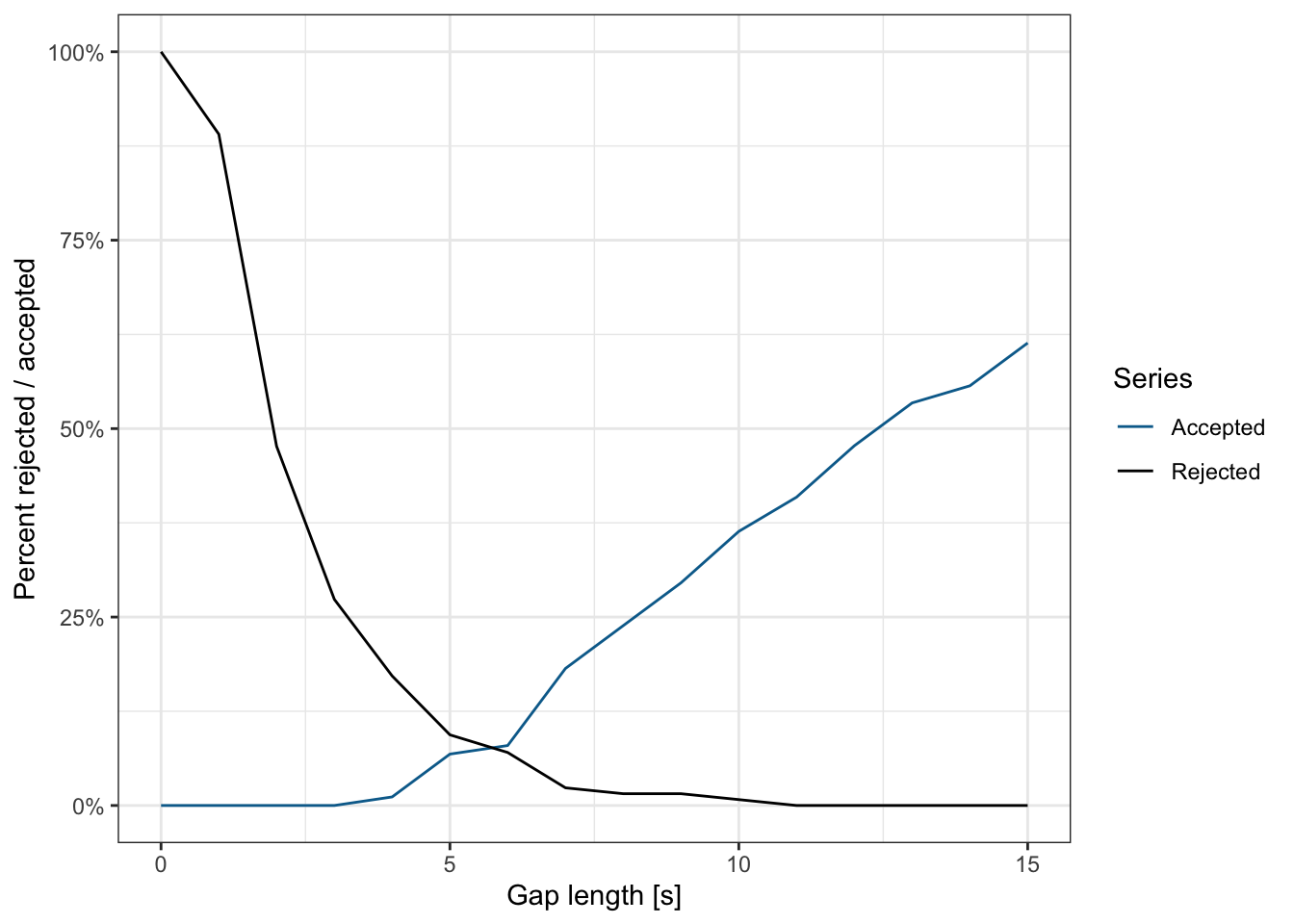
The critical gap \(t_c\) can be calculated by interpolating between the points on the two lines, \[ t_c = \frac{(t_2 - t_1)[R(t_1) - A(t_1)]}{[A(t_2) - R(t_2)] + [R(t_1) - A(t_1)]} + t_1 \tag{3.38}\]
where \(A(t)\) is the percent of accepted gaps at time \(t\), \(R(t)\) is the percent of rejected gaps, and \(t_1, t_2\) are the times bracketing the critical gap.
There are two ways to use this critical gap. First, if the critical gap is excessively long, then vehicles might not feel safe departing the intersection. Second, if the critical gap is not commonly found in the traffic streams on the major street, then you might need to interrupt the major street traffic for minor street traffic to move, i.e. with a traffic signal.
3.4.2 Approach Speed
Knowing whether to put a stop sign, yield sign, or no control at a minor street movement is a function of how well drivers approaching the intersection can see conflicting cars on the major street. This method to calculate critical approach speed (CAS) relies on identifying the distances between the approaching vehicles and the curb. 4
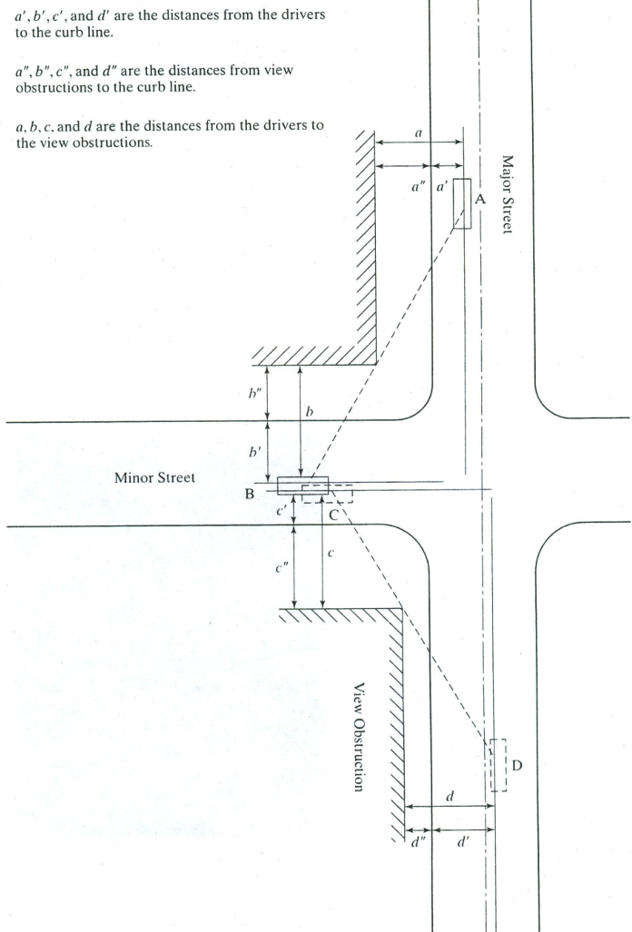
Figure 3.24 shows these distances. There are four key distances to measure, \(a, b, c, d\), each broken in two parts. The first part of each distance from the vehicle to the curb is assumed based on the roadway conditions:
- \(a\): major street, near side \(a'\): 12 feet with parking, 6 feet otherwise
- \(b\): minor street, driver side \(b' = \min(w_{min} / 2 + 3, w_{min} - 12)\) feet
- \(c\): minor street, passenger side \(c'\) = 12 feet with parking, 6 feet otherwise
- \(d\): major street, far side \(d' = w_{maj}/2 + 3\) feet
Where \(w_{min}\) and \(w_{maj}\) are the widths of the minor and major streets. The second part of the four distances is measured from the curb to any sight obstructions (buildings, trees, etc.) \(a'', b'', c'', d''\) must be measured at the site.
Once these values are obtained, the engineer makes use of the graphical tool in Figure 3.25 to determine the safe approach speed from each direction. This assumes that a vehicle on the minor street traveling below that speed would be able to stop safely after seeing a vehicle in the major street traveling at the given vehicle speed. The CAS is the smaller of the two values obtained from \((a,b)\) and \((c, d)\).
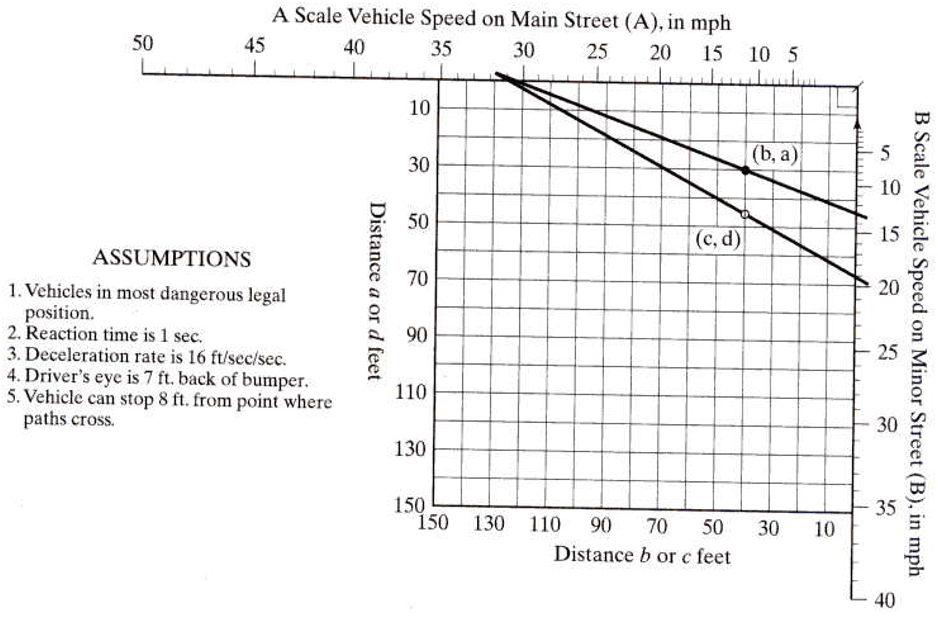
If the CAS is below 10 mph, a stop sign is required. If it is between 10 and 15 mph a yield sign might be appropriate. If it is higher than 15 mph, further study may be necessary but based on sight distances alone, an uncontrolled intersection may be feasible.
3.4.3 Roundabouts
Roundabouts are innovative unsignalized intersections where drivers yield to vehicles already in the roundabout but otherwise may proceed without stopping. The basic features of roundabouts ensure that motorists have fewer conflict points than four-way intersections. This may make roundabouts considerably safer, as motorists are less likely to miscalculate the length of a multi-directional gap. Separating the gaps and simplifying the driving task can also give roundabouts a considerably higher capacity than a four-way or two-way stop intersection, and it allows minor street movements to make left turns more easily than a two-way stop would. Roundabouts often serve as excellent passive traffic calming, and pedestrians only have to consider traffic coming from one direction at a time due to the refuge incorporated into the intersection design.
There are drawbacks to roundabouts as well. If the major street traffic has no gaps, it may be difficult for minor street movements to find gaps, and a signal might be warranted instead. Roundabouts also take more space than four-way stop intersections, meaning that they might not fit in every intersection that would benefit from one. The added space also means that pedestrians may have longer walking paths than they did previously.
Tip
Sometimes cyclists are unsure how to handle roundabouts. Remember that cyclists are vehicles: as a cyclist, you should use the full lane of the roundabout; as a motorist, treat the cyclist as any other vehicle. Unnecessarily yielding when you have the right of way creates a more dangerous situation for everyone.
3.5 Signalized Intersections
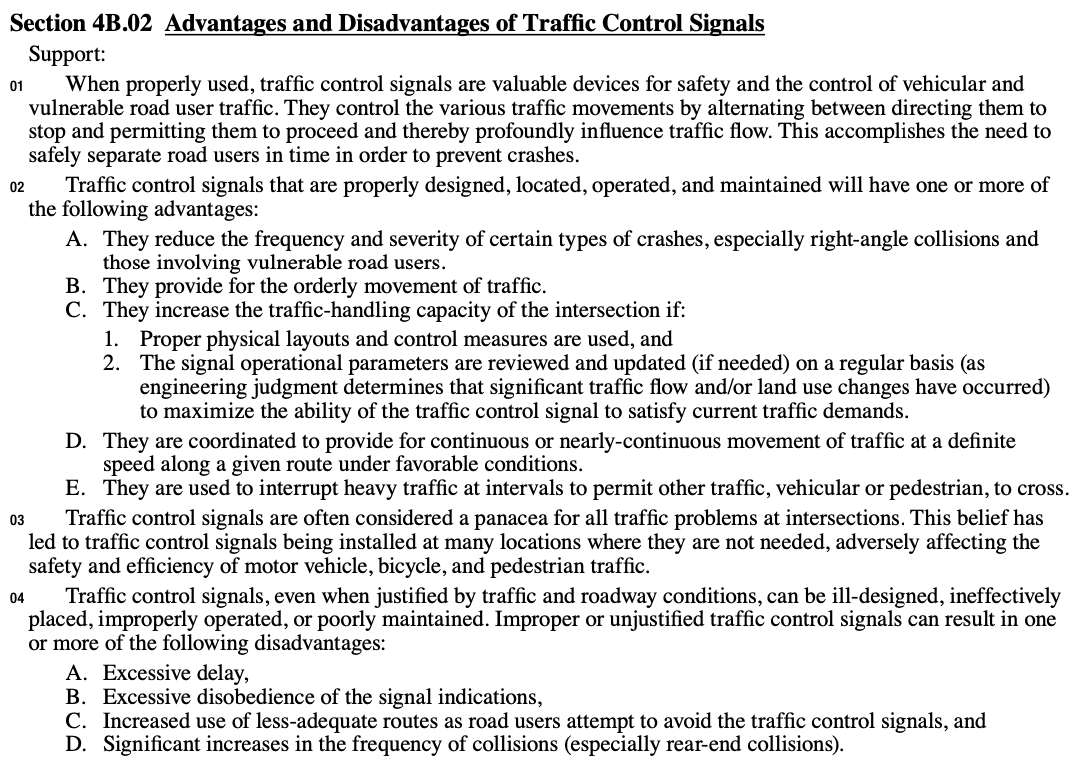
Intersections with high volumes of traffic – especially with multiple lanes – often require traffic signals to safely control intersecting traffic. The MUTCD (see Figure 3.27) describes benefits of signals: increased safety, increased flow, and orderly traffic. On the other hand, the MUTCD also points out limitations of poorly placed or timed signals, which can increase delay and reduce driver compliance.
3.5.1 Signal Warrants
Traffic signals are not cheap to install, and require periodic intervention by traffic engineers and maintenance crews to ensure they remain operational and are optimally timed for changing traffic flows. Additionally, the vehicle delay at a traffic signal with low volumes is usually longer per vehicle than at an equivalent unsignalized intersection: many of us have been the only car at an intersection while waiting for the light to change late at night.
Given these costs, signals should only be installed at intersections if there is a compelling reason to do so. The MUTCD describes a series of traffic signal warrants in Section 4C.01 with the following standard:
The investigation of the need for a traffic control signal shall include an analysis of factors related to the existing operation and safety at the study location and the potential to improve these conditions, and the applicable factors contained in the following signal warrants [see list below]. The satisfaction of a traffic signal warrant or warrants shall not in itself require the installation of a traffic signal.
There are nine warrants:
- Eight-Hour Vehicular Volume
- Four-Hour Vehicular Volume
- Peak Hour
- Pedestrian Volume
- School Crossing
- Coordinated Signal System
- Crash Experience
- Roadway Network
- Intersection Near a Grade Crossing
Each of these warrants has its own set of criteria. We will consider only the first warrant here, but all the warrants function in a similar way. The first warrant reads:
The need for a traffic control signal should be considered if an engineering study finds that one of the following conditions exist for each of any 8 hours of an average day:
- The vehicles per hour given in both of the 100 percent columns of Condition A in Table 4C-1 exist on the major-street and the more critical minor-street approaches, respectively, to the intersection; or
- The vehicles per hour given in both of the 100 percent columns of Condition B in Table 4C-1 exist on the major-street and the higher-volume minor-street approaches, respectively, to the intersection.
These major-street and minor-street volumes shall be for the same 8 hours for each condition; however, the 8 hours that are selected for the Condition A analysis shall not be required to be the same 8 hours that are selected for the Condition B analysis.
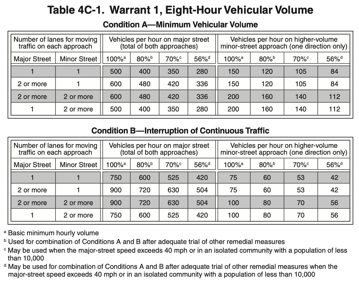
Figure 3.28 presents Table 4C-1 from the MUTCD. To use this warrant, you need to collect at least eight hours of traffic volume data. Note that the volume thresholds defined in Table 4C-1 need to be exceed in eight hours of the day, but they do not need to be consecutive.
3.5.2 Signal Terminology
Traffic signals are relatively complex devices in terms of both their electrical engineering and in how civil engineers specify and program them. This complexity requires fairly specific terminology:
- Signal Indication: The illumination of a signal lens or equivalent device.
- Interval: The part of a signal cycle during which signal indications do not change.
- Signal Phase: The green, yellow change, and red clearance intervals in a cycle that are assigned to an independent traffic movement or combination of movements.
- Cycle Length: The time required for one complete sequence of signal indications.
These elements are illustrated in Figure 3.29, called a ring barrier diagram. Most intersections have eight phases: the four through movements on each approach and the four left turns on each approach. With the left turn movements occurring before the through movements, the two rings have phases 1 through 4 and 5 through 8 proceeding in a logical order. Even at intersections where the left turns occur after the through movements, the left turns are given odd phase numbers. The primary movements at an intersection are almost always phases 2 and 6.
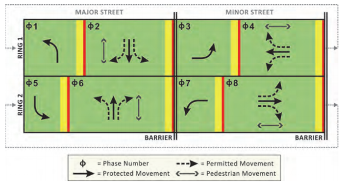
Note that within a ring and between the barriers, the intervals can be set at any length to accommodate varying traffic volumes without leading to conflicting traffic.
3.5.3 Dilemma Zones
When a signal indication changes to yellow / amber, drivers face a decision as to whether they must stop or proceed through the intersection. The distance required to stop \(x_s\) for the signal is simply the stopping sight distance formula from Equation 3.6, \[ x_s = v_0 t_r + \frac{v_0^2}{2 * d_{brake}} \tag{3.39}\] \[ x_s = v_0 t_r + \frac{v_0^2}{2 * g(f_r \pm G)} \tag{3.40}\] where \(v_0\) is an initial speed and \(d_{brake}\) is a deceleration parameter. This is a minimum stopping distance: drivers closer to the intersection than \(x_s\) cannot stop safely or comfortably, and should instead attempt to clear the intersection.
The maximum distance \(x_c\) at which a driver can clear the intersection can be described as: \[ x_c = v_0 t_y \tag{3.41}\]
where \(t_y\) is the length of the yellow interval.
Warning 3.3: Red light laws
Note that Equation 3.41 assumes that the driver will reach the stop bar on the near side of the intersection immediately at the end the yellow interval. This would then necessitate an “all red” clearance interval of \((W + L)/v_0\) — where \(W\) is the width of the intersection, and \(L\) is the length of the vehicle — to allow the vehicle to clear through the other side of the intersection before the next phase begins its green interval.
In some locations, the law require drivers to clear the intersection completely during the yellow interval. In this case, Equation 3.41 becomes \[ x_c = v_0t_y - (W + L) \tag{3.42}\] In other locations, drivers must enter the intersection before the end of the yellow interval and clear the intersection during the all-red interval. In this case, the equation becomes \[ x_c = v_0(t_y + t_{ar}) - (W + L) \tag{3.43}\] with \(t_{ar}\) the length of the all-red interval.
A dilemma zone exists when a driver cannot safely stop or clear the intersection. This exists if \(x_s > x_c\).
3.5.4 Signal Coordination
Traffic signals along a corridor often need to be coordinated so that traffic can flow smoothly. Signal coordination is almost always possible in one direction, can often be possible in two directions, but is extremely difficult in all directions on a network.
In order to coordinate the signals, it is necessary to offset the signal cycles relative to a master controller or reference intersection. A useful tool in calculating offsets and corridor progression is a time space diagram, which has time on the \(x\)- axis and space on the \(y\) axis. By drawing the cycles on the figure it is possible to determine correct offsets and corridor progression plans for vehicles of different speeds.
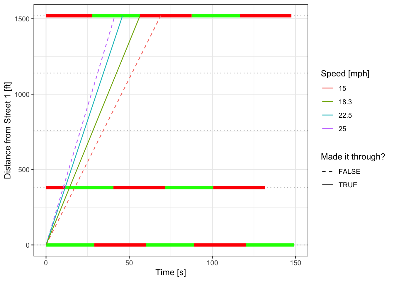
One can also use this method to look at progression in the reverse direction.
Homework
HW 3.1: Reaction Time Tests
Look on the internet to find two different reaction time tests. Try them; what is your estimated reaction time? Describe the process of each test you tried and summarize your results. Are these tests reliable? Are they an accurate way to measure your reaction speed?
HW 3.2: Visual Acuity
If a speed limit sign is 500 feet away, how tall must the letters be (in inches) for an average driver (visual acuity of 0.0019 radians) to read it?
HW 3.3: Racing a Train
Your friend makes the terrible decision to try and beat a train to the upcoming intersection. The friend is driving along a road going 65 mph, and is 500 feet from the intersection when he makes the decision. The train is 900 feet from the intersection and moving at 55 mph.
- Your friend has a reaction time of 0.8 seconds. How much distance will your friend cover while he is making the decision?
- Your friend’s car can accelerate 10 ft/sec/sec, and it has a maximum speed of 85 mph. How fast will the car be going when it reaches the intersection?
- How long did it take for your friend to reach the crossing? Did he beat the train?
HW 3.4: Stopping on a Downhill Grade
At one point on Foothill drive in Provo, there is a 3.7 percent downhill grade. What is the minimum stopping distance and time to bring a car traveling at 30 mph to a stop on that segment? Assume the driver’s reaction time is 1.8 seconds and the coefficient of rolling friction is \(f_r = 0.27\).
HW 3.5: Hitting Construction Barrels
A student is driving on a level road, and comes around a corner to see a road closure warning 520 feet away. The weather conditions consist of rain and wind. The student strikes barrels in the closed lane, but she claims that she was not violating the 55 mph speed limit and was not distracted. You are an expert witness investigating the accident and you will testify in court.
- What evidence do you need?
- What will you tell the court? Conduct an analysis of what combinations of speed, reaction times, and friction values will lead to the driver stopping in time (or not).
HW 3.6: Who must stop?
A driver approaches a stop-sign-controlled intersection from the eastbound approach. The stop sign has a supplemental sign beneath it stating “cross traffic does not stop”. Which approaches to the intersection are required to stop?
- eastbound
- northbound
- southbound
- westbound
HW 3.7: Traffic Control Devices, Lane Lines
A traffic engineer is designing new lane lines on University Avenue in Provo in a place where there is no center turn lane.
- What color should the double solid center lines be?
- What color should the dashed lines that separate lanes be?
- Many drivers on this road are cited for running red lights. A Provo city engineer wants to convert the last X feet of the dashed lane divider into a solid line. If the driver is not within that solid line zone when the light turns yellow, they should stop. Otherwise, they should continue through the intersection at the legal speed limit. If the speed limit is 40 mph, how long should the solid line be? Assume a reaction time of 2 s and the coefficient of friction \(f= 0.3\).
HW 3.8: Research On Stop Signs
Using your internet browser to search if stop signs are a good way to control speeds in residential areas. Use three credible sources to answer the following questions.
- Make a list of each reference and summarize their position on the topic.
- What is your conclusion?
- Have you personally seen stop signs effectively regulate residential speed?
- What are the pros and cons to using stop signs to control speeds in residential areas?
HW 3.9: Vehicle Speed Reduction Research
Find in the academic or professional literature an example of a traffic calming device that has been shown to significantly reduce vehicle speeds. Have you seen these devices implemented in your neighborhood? What do you think might be objections to installing them? Be sure to cite your sources.
HW 3.10: Vertical Curves
The following data describes a crest vertical curve: The VPC is at station 31 + 27 with the VPT is at station 50 + 71 with elevation 350 feet, \(G_1\) = 3 percent, and \(G_2\) = -5 percent. What is the station and elevation of the highest point of the curve?
HW 3.11: Vertical Alignment
The following data describes a sag vertical curve. The VPC is at station 23 + 79.32 and elevation 584 ft, \(L\) = 560 ft., \(G_1\) = -2 percent, \(G_2\) = 4.5 percent.
- What is the station and elevation of the lowest point of the curve?
- Find the curve’s elevation at station 24 + 00, at 26 + 00, at 28 + 00, and at the VPT. Note: It might be helpful to make a plot of the curve.
HW 3.12: Vertical SSD
A 520-foot vertical curve on an existing road has an incoming grade of \(G_1 = 3\) percent and an outgoing grade of \(G_2 = -5\). The current design speed is 55 mph. Use the default values described in Section 3.3.2.1
- Does the vertical curve currently meet minimum SSD standards?
- You wonder if lowering the design speed to 45 mph will ensure that the minimum SSD is met. Is this true?
HW 3.13: Sag Vertical Curve above a Culvert
The following data describes a sag vertical curve. \(G_1 = -3.3\) percent, \(G_2 = 4.7\) percent, the VPI is at station 50 + 00 with elevation of 532 ft. To provide proper cover over a storm drain, the elevation at station 50 + 75 needs to be 538 feet or higher.
- What is the minimum length of the curve required to provide the necessary cover? Hint: You may solve this problem by using goal seek, or by solving the curve equation for \(L\)
- Find the minimum length of curve that will provide a stopping sight distance of 600 ft. Use the default values from the text. Will this curve still clear the culvert?
HW 3.14: Horizontal Alignment
The following data describes a horizontal curve. The radius is 1,750 ft, the curve angle is 42.8 degrees, the PI is located at station 45 + 00 , and the road is a two-lane road (one 12-ft lane in each direction) with 12-foot wide lanes. Use this information to find the following:
- Degree of Curvature
- Station of PC
- Length of the curve
- Station of PT
- Middle ordinate
- Length of the chord connecting PC to PT
HW 3.15: Horizontal Curve
An exit on I-15 consists of one 12-ft lane and resembles a horizontal curve with a central angle of 70 degrees and a length of 968 ft. If the distance cleared of obstacles is 20.3 ft from the center line, what design speed was used?
HW 3.16: Horizontal Sight Distance
A horizontal curve with a radius of 1,650 feet is part of a new road with two 12-ft lanes in each direction and a 4-foot shoulder. The project manager found that there is a dense stand of trees whose edge is 20 feet from the pavement at station 32+50. The PC is at Station 28+00. If the design SSD of 780 ft is to be achieved, how much, if at all, will the edge of the trees be need to be cut back?
HW 3.17: Superelevation, R and D
Find the minimum safe radius \(R_v\) and the maximum safe degree of curvature \(D\) for each of the following scenarios (assume \(R_v = R\) for this problem). Use Table 3.4 for the \(f_{side}\) values.
- Design speed of 40 mph, \(e_{\mathrm{max}} = 0.19\) ft./ft
- Design speed of 50 mph, \(e_{\mathrm{max}} = 0.08\) ft./ft
- Design speed of 65 mph, \(e_{\mathrm{max}} = 0.05\) ft./ft.
HW 3.18: Superelevation on State Street
The turn in South State street in Provo is in poor condition and is experiencing increasing traffic. UDOT would like to build a superelevated curve at this intersection5 with a radius of 350 ft to the centerline. The design speed for this curve is 40 mph.
- What value of \(e_{max}\) do you recommend for this curve?
- If \(e_{max}\) = 0.07, what speed limit should be placed on the curve?
TipSolution idea
This problem doesn’t have a straightforward solution. You can iterate to a solution by first finding the speed with a given friction factor, and then updating the friction factor based on the speed.
HW 3.19: Gap Events
| Event | Time (seconds) |
|---|---|
| Major street vehicle passes through intersection | 3.1 |
| First minor street vehicle reaches head of queue | 10.4 |
| Major street vehicle passes through intersection | 14.4 |
| Major street vehicle passes through intersection | 17.0 |
| Major street vehicle passes through intersection | 18.8 |
| First minor street vehicle turns through intersection | 19.4 |
| Second minor street vehicle reaches head of queue | 25.0 |
| Second minor street vehicle turns through intersection | 26.0 |
| Third minor street vehicle reaches head of queue | 30.2 |
| Major street vehicle passes through intersection | 33.4 |
| Major street vehicle passes through intersection | 37.5 |
| Third minor street vehicle turns through intersection | 39.1 |
| Major street vehicle passes through intersection | 52.1 |
Table 3.8 shows a sequence of vehicle events at a T-intersection. Calculate the length of each gap, and identify whether the gap was accepted or rejected. Show your calculations. Note: Assume the minor street vehicle has not passed through the intersection until it is explicitly stated that it has.
HW 3.20: Estimating Critical Gaps
Table 3.9 below shows the number of cars observed to accept or reject gaps of at least a particular length at a particular intersection. That is, the 18 vehicles that accept a gap of at least 7 seconds includes the 14 vehicles that accepted a gap of at least 6 seconds. A CSV file of the data is available here. Note: You should use a spreadsheet to solve this problem, but document your work with example calculations and do not submit merely a workbook.
- Compute the proportion of drivers that accept a gap of each length.
- Compute the proportion of drivers that reject a gap of each length.
- Plot the proportions calculated in part a and part b.
- Estimate the critical gap to the nearest tenth of a second.
| Gap Length [s] | N Accepted (less than gap) | N Rejected (less than gap) |
|---|---|---|
| 1 | 0 | 145 |
| 2 | 1 | 125 |
| 3 | 2 | 63 |
| 4 | 6 | 34 |
| 5 | 8 | 20 |
| 6 | 14 | 7 |
| 7 | 18 | 5 |
| 8 | 28 | 2 |
| 9 | 33 | 2 |
| 10 | 42 | 2 |
| 11 | 47 | 1 |
| 12 | 52 | 0 |
HW 3.21: Critical Approach Speed Analysis
There is an intersection on UT route 189 that has had a large number of car crashes, and limited sight distance is a potential cause. The 85th percentile speed is 48 mph. The highway is 76 feet wide; the road that it intersects with is 48 feet wide. Parking is permitted on both sides of both streets. The distances from curb to the obstruction are given as:
- \(a''\) = 40 feet
- \(b''\) = 73 feet
- \(c''\) = 94 feet
- \(d''\) = 85 feet
Calculate the critical approach speed at the intersection. Show your calculations of the geometry as well as your copy of the critical approach speed graphic. What traffic control devices should be placed at the intersection?
HW 3.22: Critical Approach Speed
The 85th percentile speed on a major street is 31 mph. Parking is prohibited on the Major Street, but it is allowed on the Minor Street. The Major Street is 60 feet wide and Minor Street is 36 feet wide. The distances from curb to view obstruction, are: \(a” = 24\) feet, \(b” = 19\) feet, \(c” = 28\) feet, \(d” = 12\) feet.
- Determine the CAS and whether a stop sign or yield sign is indicated.
- How high must the approach speed on 8th Ave. be, so that a stop sign on the minor is required? Explain your answer.
- What if parking is no longer permitted on the minor street? Will the traffic control device change? change?
- If the 85th percentile speed on the major street had been 39 mph, rather than 31 mph, what traffic control device would be appropriate?
- If \(a”\) and \(c”\) were both 16 ft, what traffic control device would be needed with the speed on the major street at 31 mph?
HW 3.23: Traffic Signal Warrants
Repeat the analysis in the example in Section 3.5.1, this time with using 2 lanes on the minor street instead of one lane. Do any results change? Provide any calculations and a summary of what you found.
HW 3.24: Dilemma Zones
An approach to an intersection with a 55 mph speed has a yellow interval length of 4 seconds. Assume a reaction time of 2 seconds and a deceleration of 10 \(ft/s^2\). The intersection is 100 feet wide and the high percentage of trucks means that the average vehicle length is 32 feet.
- Show if a dilemma zone exists, and determine how long it is
- What should be time for the all-red interval on this phase?
- What should be length of the yellow interval so that a dilemma zone no longer exists?
HW 3.25: Traffic Signal Timing
| Interval | NB Left Turn | NB Through and right turn | SB Vehicles | EB Vehicles | WB Vehicles |
|---|---|---|---|---|---|
| 1 | G=9 | G=52 | R=13 | R=56 | R=56 |
| 2 | Y=3 | ||||
| 3 | R=85 | ||||
| 4 | G=39 | ||||
| 5 | Y=3 | Y=3 | |||
| 6 | R=42 | R=42 | |||
| 7 | G=37 | G=37 | |||
| 8 | Y=3 | Y=3 | |||
| 9 | R=1 | R=1 |
Table 3.10 shows the timing pattern at a traffic signal in Provo. Complete the following regarding traffic signal timing.
- In the diagram shown above how many EB phases are there?
- How many intervals are there during the time that NB through and right turn traffic sees green?
- What is the length of the all-red clearance interval?
- Draw a ring barrier diagram for the traffic signal. It should be roughly to scale, and identify the phase numbers assigned to each movement.
HW 3.26: Time Space Diagram
| Cycle | Green Start |
|---|---|
| Center Street | |
| 1 | 17:14:11 |
| 2 | 17:15:26 |
| 3 | 17:16:41 |
| 500 North | |
| 1 | 17:22:03 |
| 2 | 17:23:18 |
| 3 | 17:24:33 |
| Cougar Blvd | |
| 1 | 17:33:06 |
| 2 | 17:34:21 |
| 3 | 17:35:36 |
You use a watch to mark the beginnings of the green phases at three intersections on University Avenue. The green phases on Center Street, 500 North, and Cougar Blvd are spaced 1,000 feet apart from each other and you mark them as starting at the times given in Table 3.11 above. Each green phase is 40 seconds long.
- What is the cycle length?
- If the master controller is at Center Street, what are the offsets at 500 North and Cougar Blvd?
- If a driver crosses University Ave at the start of that signal’s green phase and is not impeded by other traffic, what range of speeds will permit her to proceed through the green phase at 500 North without delay?
- Draw a time-space diagram for this corridor. Draw the diagram with attention to scale. Include vehicle paths for cars proceeding in the northbound and southbound direction at 30 miles per hour. Does corridor progression work in both directions?
References
1983 Traffic Control Devices Handbook : U.S. Department of Transportation : Free Download, Borrow, and Streaming : Internet Archive — archive.org. https://archive.org/details/1983-traffic-control-devices-handbook/page/2-18/mode/2up.
All images in this section are drawn from the MUTCD.↩︎
Not to be confused with the ratio of peak hour to daily traffic in Equation 2.3↩︎
The 100 scalar in the equation is a hint that the grades have been multiplied by 100↩︎
This method is described in 1983 Traffic Control Devices Handbook ↩︎
This is a made-up scenario, UDOT has no plans to do this.↩︎