4 Pavement Design and Management
In this chapter you will learn how to
- Identify two different pavement types and common distresses for each type
- Calculate the traffic demand on a pavement structure throughout a design period
- Design flexible pavements using the AASHTO Pavement Design Guide
- Manage pavement networks cost-effectively
- Perform life-cycle cost analyses for transportation facilities
4.1 Pavement Performance
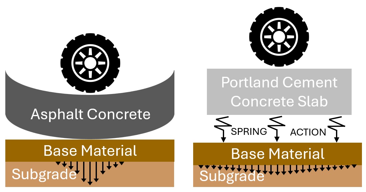
As illustrated in Figure 4.1, there are two main types of pavements:
- Flexible pavements have an asphalt concrete (AC) surface, which flexes, or bends, under traffic loads – hence the term flexible pavement.
- Rigid pavements have a portland cement concrete (PCC) surface, which displaces as a plane under traffic loads and springs back after the load is removed.
Because of their high stiffness, rigid pavements distribute traffic loads over a larger area of the underlying subgrade. In contrast, flexible pavements distribute traffic loads over a smaller subgrade area.
Pavement structures consist of multiple layers of pavement materials. For flexible pavements, the top layer, or wearing course, is asphalt concrete. Asphalt concrete is composed of asphalt binder and coarse and fine aggregate. The underlying layer is called the base layer and is typically composed of aggregate that may or may not be stabilized with chemical additives, such as portland cement concrete, to achieve greater strength. An additional aggregate layer beneath the base layer is sometimes used and is called the subbase. It is typically used to protect frost-susceptible subgrade soils in cold regions, or to protect soft clays from deformation under traffic. Finally, the lowest layer is the native soil, or subgrade.
4.1.1 Pavement Distresses
A pavement’s condition deteriorates over time as it is exposed to environment, carries traffic loads, and sustains material degradation over time. Pavement distresses are visible evidence of pavement deterioration.
4.1.1.1 Asphalt Pavement Disresses
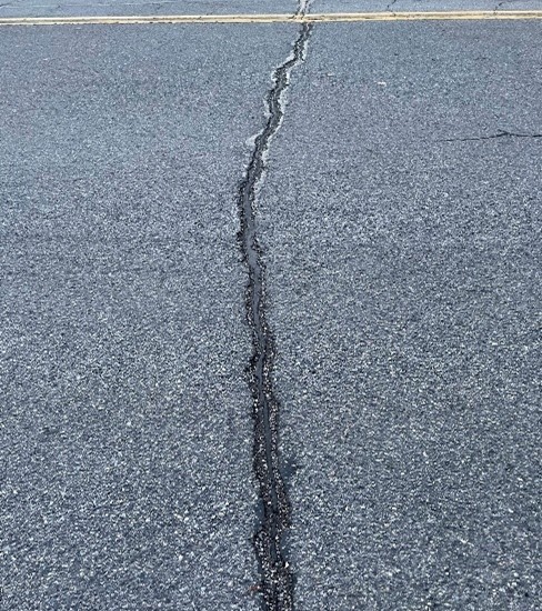
Longitudinal and Transverse Cracking Longitudinal cracks occur in wheel paths as the result of traffic loading and often occur at paving joints due to poor construction. Transverse cracks are typically environmental distresses resulting from temperature fluctuations that cause the asphalt to expand and contract.
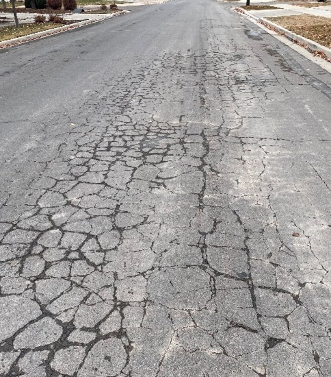
Block Cracking Block cracking is an environmental distress consisting of a network of large square or rectangular patterns. Similar to transverse cracking, it is caused temperature fluctuations.
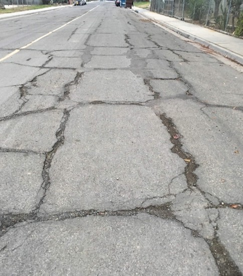
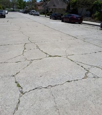
Alligator Cracking Alligator cracking is a load-related distress also known as fatigue or structural cracking. The network of cracks resembles the back of an alligator. For thin asphalt layers, it typically initiates at the bottom of the asphalt layer and propagates upward.
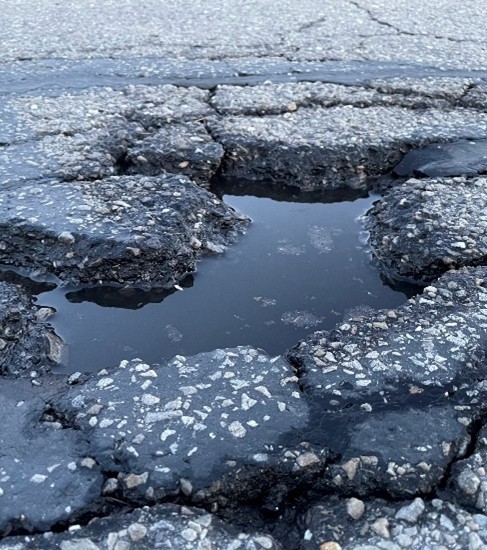
Potholes Potholes are holes in the asphalt pavement. This load-related distress typically develops from severe alligator cracking, where traffic loads cause broken pieces of asphalt to dislodge from the pavement structure.
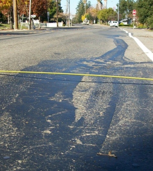
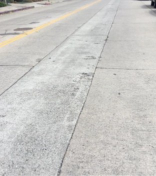
Pumping Pumping is the ejection of water and fine soil material upwards through cracks under moving loads. It is characterized by the fines on the surface of the asphalt. This distress is evidence of load-related damage and base material failure.
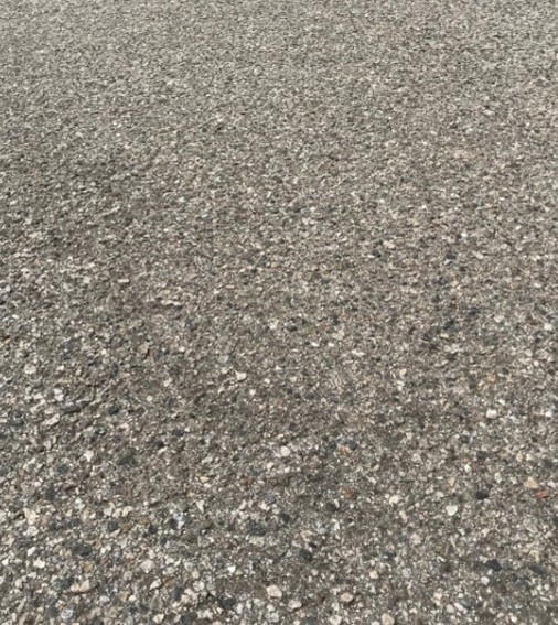
Weathering Weathering is the degradation of the asphalt surface caused by exposure to environmental factors such as sunlight. Weathered asphalt appears gray and exhibits a loss of asphalt binder such that fine aggregate is exposed on the pavement surface.
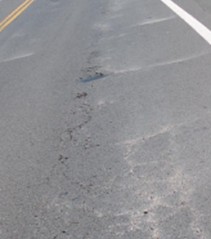
Rutting/Depression Rutting/depressions are distresses caused by a downward displacement of the pavement from it original grade. Rutting occurs longitudinally in the wheel paths, while depressions occur elsewhere. Rutting is typically a load-related distress, but in some cases indicates inadequate asphalt material stability.
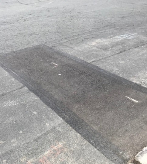
Patching and Utility Cut Patch Patching is the replacement of discrete pavement areas to either repair damaged pavement or restore pavement following subsurface utility work. Water entry and poor compaction of patches can accelerate patch deterioration.
4.1.1.2 Portland Cement Concrete Pavement Disresses
Common portland cement concrete pavement distresses are shown and described below.
Corner Break A corner break is a vertical crack that intersects perpendicular edges of a slab. It is typically caused by inappropriate joint spacing, load repetitions, a loss of base support, and poor load transfer across the joint.
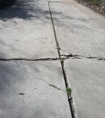
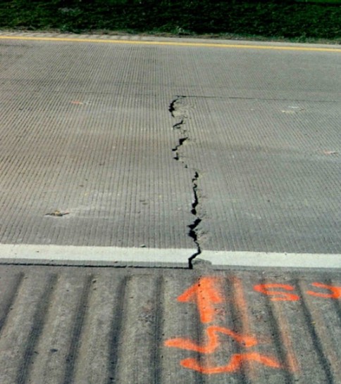
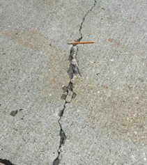
Linear Cracking Linear cracking includes longitudinal, transverse, and diagonal cracks that divide a slab into 2-3 pieces. It is typically caused by improper jointing or repeated loading.
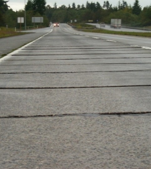
Faulting Faulting is a difference in elevation across a joint or crack, which often causes a thumping sound when traversed by a vehicle. It is caused by poor load transfer across the joint and migration of base material.
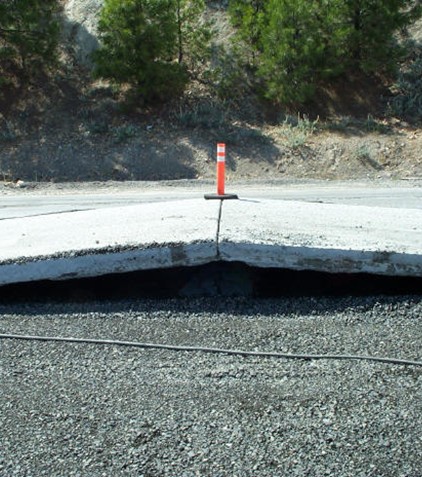
Blowups Blowups occur during high temperatures when joints are unable to accommodate the resulting slab expansion. When incompressible debris enters a joint, the expansion pressure cannot be relieved, and the slabs displace upward.
Spalling Spalling is the breakdown, or crumbling, of the slab at a joint, corner, or crack. Spalls typically occur at an angle through the concrete rather than vertically.
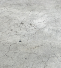
Scaling or Map Cracking Map cracking is a network of fine, shallow cracks on the concrete surface that are typically caused by poor curing or undesirable chemical reactions within the concrete. Scaling, which is when the surface of the concrete flakes off, can be caused by poor finishing or curing.
Divided Slab A divided, or shattered, slab is divided into 4+ pieces.
Patching and Utility Cuts Patching is the replacement of discrete pavement areas to either repair damaged pavement or restore pavement following subsurface utility work. Water entry and poor compaction of patches can accelerate patch deterioration.
4.1.2 Pavement Condition Indices
Pavement condition data are typically represented at one of two levels: 1) individual pavement distress type, severity, and extent or 2) overall condition for a pavement segment in terms of a composite index or rating. Common composite pavement condition assessment methods include the following:
- Present Serviceability Index (PSI)
- Pavement Condition Index (PCI)
- International Roughness Index (IRI)
- Pavement Surface Evaluation and Rating (PASER)
These indices are briefly described below.
Present Serviceability Index (PSI) Serviceability is a measure of ride quality that represents a pavement segment’s ability to serve traffic. The concept of serviceability was developed in the 1950s and 60s during the American Association of State Highway Officials (AASHO) Road Test in which a panel rated the drive quality of 74 asphalt pavement segments and 49 concrete pavement segments on a serviceability scale. The scale — shown in Table 4.1 — ranged from 0 to 5, where a rating of 5 represents a pavement segment in very good condition and a rating of 0 represents a pavement segment in very poor condition.
| Present Serviceability Index (PSI) Range | Rating |
|---|---|
| 4-5 | Very Good |
| 3-4 | Good |
| 2-3 | Fair |
| 1-2 | Poor |
| 0-1 | Very Poor |
Pavement Condition Index (PCI) In the 1970s, the United States Army Corps of Engineers developed a method1 and pavement condition index (PCI) for quantifying the overall condition of a pavement segment. The method involves a complex process for accounting for the type, severity, and extent of visible pavement distresses. As shown in Table 4.2, PCI values range from 0 to 100, with higher values representing pavements in better condition and lower values representing pavements in poorer condition.
| Pavement Condition Index (PCI) Range | Rating |
|---|---|
| 85-100 | Excellent |
| 70-85 | Good |
| 50-70 | Fair |
| 25-50 | Poor |
| 0-25 | Failed |
International Roughness Index (IRI) Pavement roughness is considered the most important indicator of ride quality by the traveling public and describes the longitudinal profile in the wheel paths of a pavement segment. The international roughness index (IRI), developed in 1980s, is defined as the ratio of the accumulated vertical suspension motion of a standard quarter-car traveling at a speed of 50 mph to the horizontal distance traveled2. The result is in units of inches per mile, where lower values describe smoother roads, and higher values describe rougher roads. Table 4.3 lists commonly observed IRI ranges for various roadway categories.
| Roadway Category | Rating |
|---|---|
| Airport runways and superhighways | $<$ 130 |
| New pavements | 100-220 |
| Older pavements | 160-380 |
| Maintained unpaved roads | 220-630 |
| Damaged pavements | 250-700 |
| Rough unpaved roads | $>$500 |
Pavement Surface Evaluation and Rating (PASER) The pavement surface evaluation and rating (PASER) method was developed in the early 2000s. This visual inspection assigns a condition rating to a pavement segment based on observed distresses and requires no calculations, making it a practical option for local agencies with limited resources, funds, and personnel. Ratings range from 10 to 1, with a rating of 10 representing a new pavement and a rating of 1 representing a structurally failed pavement. Table 4.4 lists the good, fair, and poor condition categories corresponding to PASER values.
| PASER Range | Category |
|---|---|
| 8-10 | Good |
| 5-7 | Fair |
| 1-4 | Poor |
4.2 Traffic Loads
Traffic is the most important factor in pavement design. Traffic loads represent the demand that the pavement structure must be able to carry. The load placed on a road by traffic depends on vehicle weight and axle configuration (single, tandem, tridem). Heavier vehicles with fewer axles produce higher loads on the pavement.
An 18,000lb-load on a single axle is commonly used as the standard to which all other axle loads and configurations are compared and is called an Equivalent Single Axle Load (ESAL). The equivalent axle load factor (EALF), or the equivalent number of ESALs caused by a single axle carrying any load can be approximated as \[ EALF_{\mathrm{single}} = \left(\frac{W_{\mathrm{single}}}{18000}\right)^4 \tag{4.1}\] where \(W_{\mathrm{single}}\) is the weight loaded at each single axle. Equation 4.1, is also sometimes called the “fourth power formula” after its mathematical form.
An EALF can be computed for each axle configuration on a vehicle, and the sum of the EALFs for a given vehicle then represents the total number of ESALs for that vehicle, which is also known as the truck factor. For heavy-duty tractors (semi-trucks), typical loads on steering axles are between 10,000 and 12,000 lb and the maximum gross vehicle weight in most states in the U.S. is 80,000 lb.
NoteFive Axle ESAL
The five-axle heavy-duty tractor-trailer shown below is loaded to the legal limit of 80,000 lb. In this configuration, a tractor with two axles is pulling two trailers, the first with a single rear axle and the second with single front and rear axles. The total load is distributed such that the front axle carries 12 kips (1 kip = 1000 lb) while each of the other axles carries 17 kips.
What is the total ESAL value, or truck factor, for this vehicle?
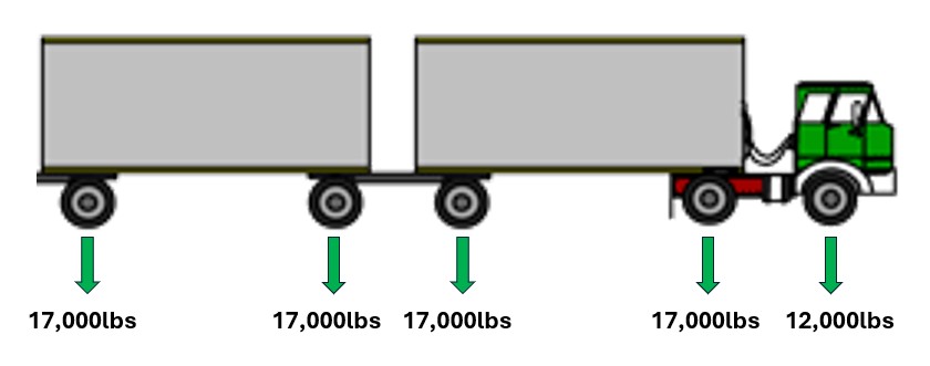
Applying Equation 4.1 to each of the vehicles axles and then summing yields
\[\begin{align*} \mathrm{Truck \ Factor}&= \sum_{i = 1}^n \left(\frac{W_{\mathrm{single}}}{18000}\right)^4\\ &= \left(\frac{12000}{18000}\right)^4 + 4 \times \left(\frac{17000}{18000}\right)^4\\ &= 3.38 \end{align*}\]
Each truck with this configuration adds 3.38 ESALs to the total pavement load.
When two axles are adjacent, called tandem axles, they function as a unit and reduce the resulting damage to the pavement. The fourth power formula for computing an EALF for tandem axles is:
\[ EALF_{\mathrm{tandem}} = \left(\frac{W_{\mathrm{tandem}}}{33200}\right)^4 \tag{4.2}\]
Note18-wheeler ESAL
A standard tractor semi-trailer vehicle (commonly called an 18-wheeler) has the axle load configuration shown when fully loaded (80,000 lb gross vehicle weight).
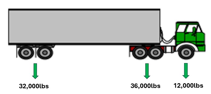
What is the total ESAL, or truck factor, for this vehicle?
Using Equation 4.1 and Equation 4.2 and summing, we get, \[\begin{align*} \mathrm{Truck \ Factor} &= \left(\frac{12000}{18000}\right)^4 + \left(\frac{36000}{33200}\right)^4 + \left(\frac{32000}{33200}\right)^4\\ &= 2.44 \end{align*}\]
Therefore, one pass of this 18-wheeler causes the same amount of damage as 2.44 passes of an ESAL, which is only \(2.44/3.38=72\%\) of the damage caused by the 5-axle truck in the previous example, even though the total weight of the vehicle is the same.
Similarly, three adjacent axles, called tridem axles, also function as a unit and reduce the resulting damage to the pavement. The fourth power formula for computing an EALF for tridem axles is \[ EALF_{\mathrm{tridem}} = \left(\frac{W_{\mathrm{tridem}}}{47600}\right)^4 \tag{4.3}\]
A typical passenger car weighs approximately 3,000 lb, which corresponds to a total ESAL value, or truck factor of 0.0001. One pass of the fully loaded 18-wheeler described in the previous example therefore causes the same amount of damage as \(2.44/0.0001 = 24,400\) passes of a typical passenger car! Because the relative damage a typical passenger car causes to a pavement structure is negligible when compared to the damage caused by truck traffic, truck traffic is considered during pavement design, while passenger traffic damage is typically ignored.
To obtain the design ESALs, or traffic demand that a pavement must carry, the current truck traffic mix (types and numbers per year) must be estimated. For each combination of axle configuration and weight, the EALF value is calculated and multiplied by the annual number of passes of that axle expected during the first year of the pavement service life. Those products are then summed to obtain the total annual ESALs for that first year. This value is then projected based on an expected annual traffic growth rate through the pavement service life, \[ ESAL_{\mathrm{design}} = ESAL_{\mathrm{first\ year}} \left[\frac{(1 + r)^Y - 1}{r}\right] \tag{4.4}\] where \(r\) is the growth rate and \(Y\) is the number of years in the design period.
Tip
Note that this is the standard \(F = A(i, n)\) equation (future value of a repeating value for \(n\) periods).
TipESALs in practice
For large, federally funded roads in the United States, current practice has progressed / advanced beyond the ESAL method. AASHTO publishes both charts and software that allows engineers to forecast pavement traffic loading as a result of vehicle counts and an understanding of pavement mechanics. The ESAL method is still used in cities and counties — and internationally. It also provides a good introduction to more advanced methods you might encounter later, specifically in CE 563
4.3 Soil Characteristics
The native soil on which a pavement is built is called subgrade when it functions as the lowest layer in a pavement structure. The soil properties heavily influence the load-carrying capacity of the pavement. Organic soils are highly compressible and susceptible to frost effects and are therefore totally unsuitable as pavement base layers. Poor soil materials are typically removed from the road site and replaced with higher-quality, well-graded gravel materials. In general, coarse-grained soils (gravels) exhibit higher bearing capacity, while fine-grained soils (sands, silts, and clays) exhibit lower bearing capacity. The quality of drainage typically decreases with increasing percentages of finer soil particles. Because the particle size distribution and fines content of aggregate materials can be controlled, aggregate layers can be engineered for use as base and subbase layers in pavement structures.
A soil’s resilient modulus \(M_R\) is a measure of its structural capacity. Similar to the modulus of elasticity, \(M_R\) is a stress divided by a strain and has the units of pounds per square inch, or psi. This value is obtained from a laboratory test in which a cylindrical specimen is repeatedly loaded and unloaded axially, to simulate repeated wheel loads, while the deformation is measured. After a specified number of load cycles, the stress is computed by dividing the applied load by the initial cross-sectional area of the specimen, and the strain is computed by dividing the recoverable deformation by the initial specimen height. A soil’s \(M_R\) value is temperature and moisture-dependent and therefore varies throughout the year. Table 4.5 shows typical resilient modulus values for various soil types.
| Material | $M_R$ (psi) |
|---|---|
| Crushed Stone | 20,000 - 40,000 |
| Sandy Soil | 7,000 - 30,000 |
| Silty Soil | 5,000 - 20,000 |
| Clay Soil | 5,000 - 15,000 |
| Organic | $<$ 5,000 |
A soil’s California Bearing Ratio (CBR) is also a measure of its structural capacity. The CBR value is a ratio of the bearing capacity of a soil to the bearing capacity of a reference well-graded crushed stone defined to have a CBR of 100%. For low CBR values (less than 20), \(M_R\) can be estimated according to the following relationship: \[ M_R = 1500\times CBR \tag{4.5}\]
4.4 Flexible Pavement Design
Pavement design is based on the structural principle of providing sufficient structural capacity to withstand the traffic demand over the design period. As with all structures, the capacity must exceed the demand.
Tip
This course only covers the AASHTO Pavement Design method for flexible pavements. Other flexible pavement design methods — as well as rigid pavement design methods — are covered in depth in CE 563.
4.4.1 Structural Number
The structural number (SN) of a pavement represents the structural capacity of all pavement layers (excluding the subgrade) to withstand traffic loading. The higher the SN, the greater the structural capacity. The SN for a pavement structure is: \[ SN = a_1 d_1 + a_2 d_2 m_2 + a_3 d_3 m_3 \tag{4.6}\] where \(a_1, a_2, a_3\) are the structural coefficients for the asphalt, base, and subbase materials, respectively; \(d_1, d_2, d_3\) are the thicknesses (in inches) of those same layers; and \(m_2\) and \(m_3\) are the drainage coefficients for the base and subbase layers (the drainage coefficient of asphalt is 1).
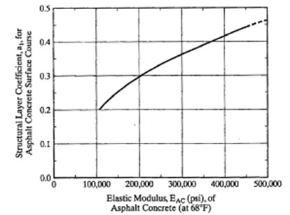
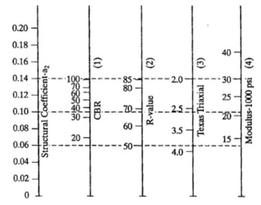
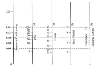
The structural coefficients, or the \(a\) variables, represent the structural capacity per vertical inch of material. Structural coefficients are not measured directly but can be inferred from various laboratory tests. For example, if the resilient modulus of an asphalt is known, it can be correlated to the structural coefficient, \(a_1\), using Figure 4.18 in which a horizontal line drawn across the figure intersects the vertical scales at equivalent values. Similar correlation charts for base and subbase materials are presented in Figure 4.19.
The drainage coefficients, the \(m\) variables in Equation 4.6, represent the quality of drainage of the underlying pavement layers. If drainage is poor, such that more moisture present, the \(m\) value will be lower. Use \(m = 1\) if no information is specified.
Moisture is the enemy of pavements. Consequently, good drainage is a necessity. Moisture in underlying pavement layers weakens the pavement, exacerbates distresses, and can shorten the service life of a pavement if not accounted for in the pavement design process.
4.4.2 AASHTO Design Equation
The AASHTO Guide for Design of Pavement Structures (1993) presents the AASHTO pavement design equation, which ensures that a pavement will have a structural capacity greater than the traffic demand. This equation was developed from data collected during the AASHO road test and includes several design variables, including the SN.
\[
\log_{10}(W_{18}) = Z_R S_0 + 9.36 \log_{10}(SN + 1) - 0.2 +
\frac{\log_{10}(\Delta PSI) / 2.7}{0.4 + (1094 / (SN + 1)^{5.19})} +
2.32 \log_{10}(M_r) - 8.07
\tag{4.7}\] where:
- \(W_{18}\): the expected ESALs in millions
- \(Z_R\): pavement reliability expectation. For major roads, this will be over 90%.
- \(S_0\): standard deviation of all factors in the design: if we are more certain about \(W_18\) and the other parameters, this can be smaller. A value around 0.4 is typical.
- \(M_R\): the road bed resilient modulus in ksi.
- \(\Delta PSI\): What is the allowable deterioration in pavement serviceability over the life of the pavement?
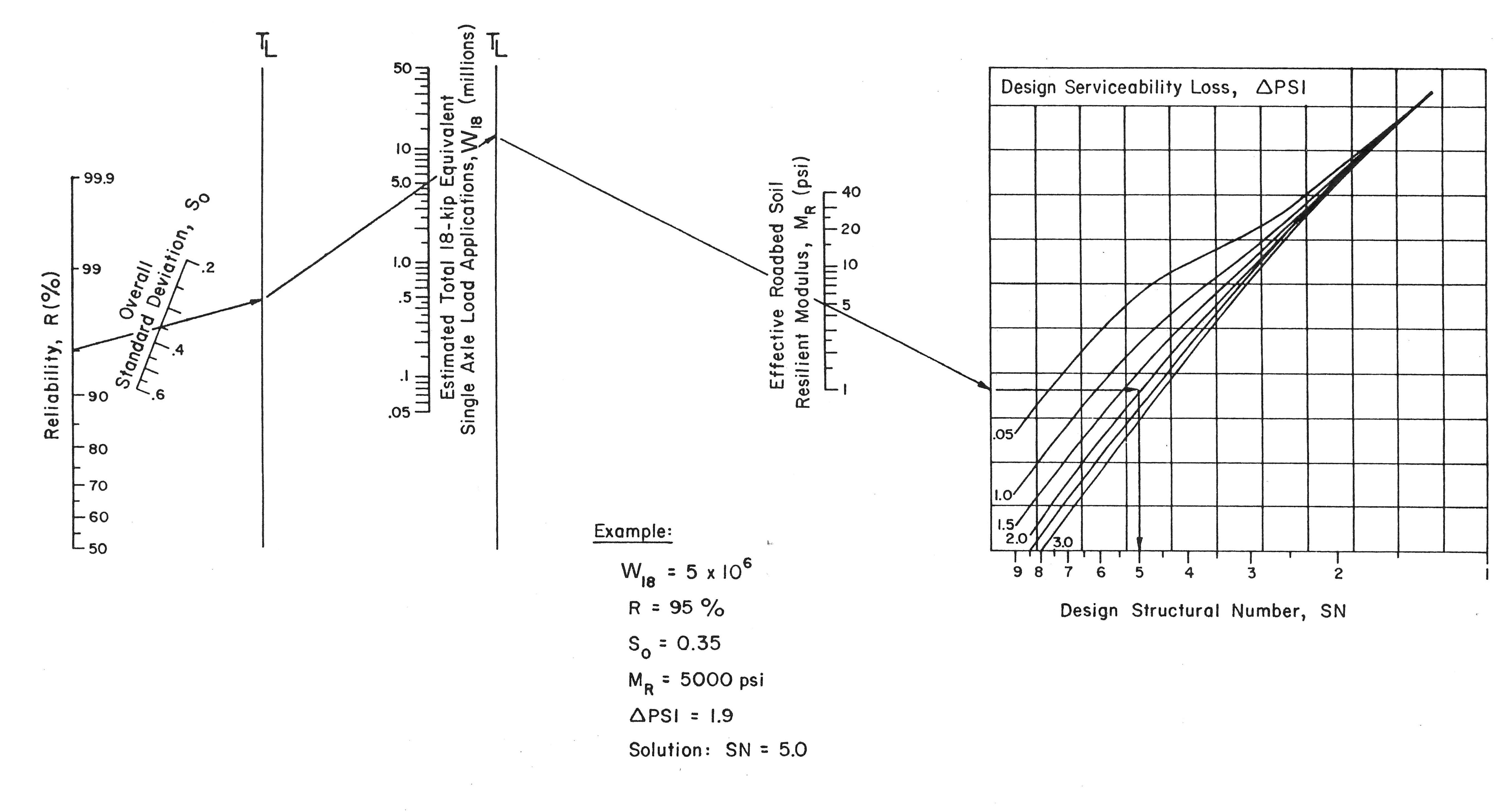
This complex equation has been reduced to the nomograph in Figure 4.20. A nomograph is a diagram prepared to allow approximate graphical solutions to an equation.
The steps to determine the structural number required for a given pavement design are as follows:
- Identify the reliability on the left vertical line in the nomograph.
- Draw a line from the reliability through the standard deviation to the first turning line (TL).
- Draw a line from the first TL through the design ESAL value to the second TL.
- Draw a line from the second TL through the subgrade MR to the left edge of the grid.
- Draw a horizontal line from the left edge of the grid to the line corresponding to the allowable serviceability loss (\(\Delta PSI\)).
- Draw a vertical line from the intersection of the previously drawn horizontal line and the allowable PSI loss down to the horizontal axis of the grid. Read the SN from the horizontal axis (note that the SN scale increases from right to left).
4.4.3 Layered Analysis
Once the SN for the overall pavement structure has been determined and the types of pavement layers have been selected for a given design, we can determine the thickness of each pavement layer using layered analysis.
Layered analysis is based on the principle that each pavement layer must protect the underlying layers. Conveniently, we can continue to use the AASHTO nomograph to determine the SN of each pavement layer (or combinations or pavement layers) that is required to protect each underlying layer. For example, to obtain the requisite SN for the asphalt layer (which protects the base layer), the resilient modulus of the base material would be used in the AASHTO nomograph. Similarly, to obtain the requisite SN for the asphalt and base layers (which together protect the subbase layer), the resilient modulus of the subbase material would be used in the AASHTO nomograph. If a material has a modulus above 40 ksi, it does not need a calculated amount of protection, and the thickness of the overlying layer(s) may be specified as the minimum per Table 4.6
| Traffic (ESAL) | HMA (inches) | Aggregate Base |
|---|---|---|
| <50k | 1.0 | 4 |
| 50k - 150k | 2.0 | 4 |
| 150k - 500k | 2.5 | 4 |
| 500k - 2 million | 3.0 | 6 |
| 2 million to 7 million | 3.5 | 6 |
| Over 7 million | 4.0 | 6 |
Layered analysis is illustrated in the following example.
NoteLayered Analysis
The pavement described in the previous example has a base layer with a resilient modulus of 25 ksi and a sub-base layer with a resilient modulus of 11 ksi. What are the SN values required to protect these layers?
The total pavement SN was found in the previous example to be 5. Since we are still working with the same overall pavement structure, the demand, reliability, and standard deviation remain the same. Therefore, because Steps 1-3 are the same as th eprevious example, we can pick up at Step 4 to determine the SN for the top two pavement layers, which protect the subbase layer. This is shown in red in the image below:
- Draw a line from the second \(T_L\) through the subbase resilient modulus value of 11 ksi to the left edge of the grid.
- Draw a horizontal line from the left edge of the grid to the curve representing the design serviceability loss of 2.0.
- Draw a vertical line dropping from the allowable PSI loss intersection down to the horizontal axis of the SN grid and read the SN.
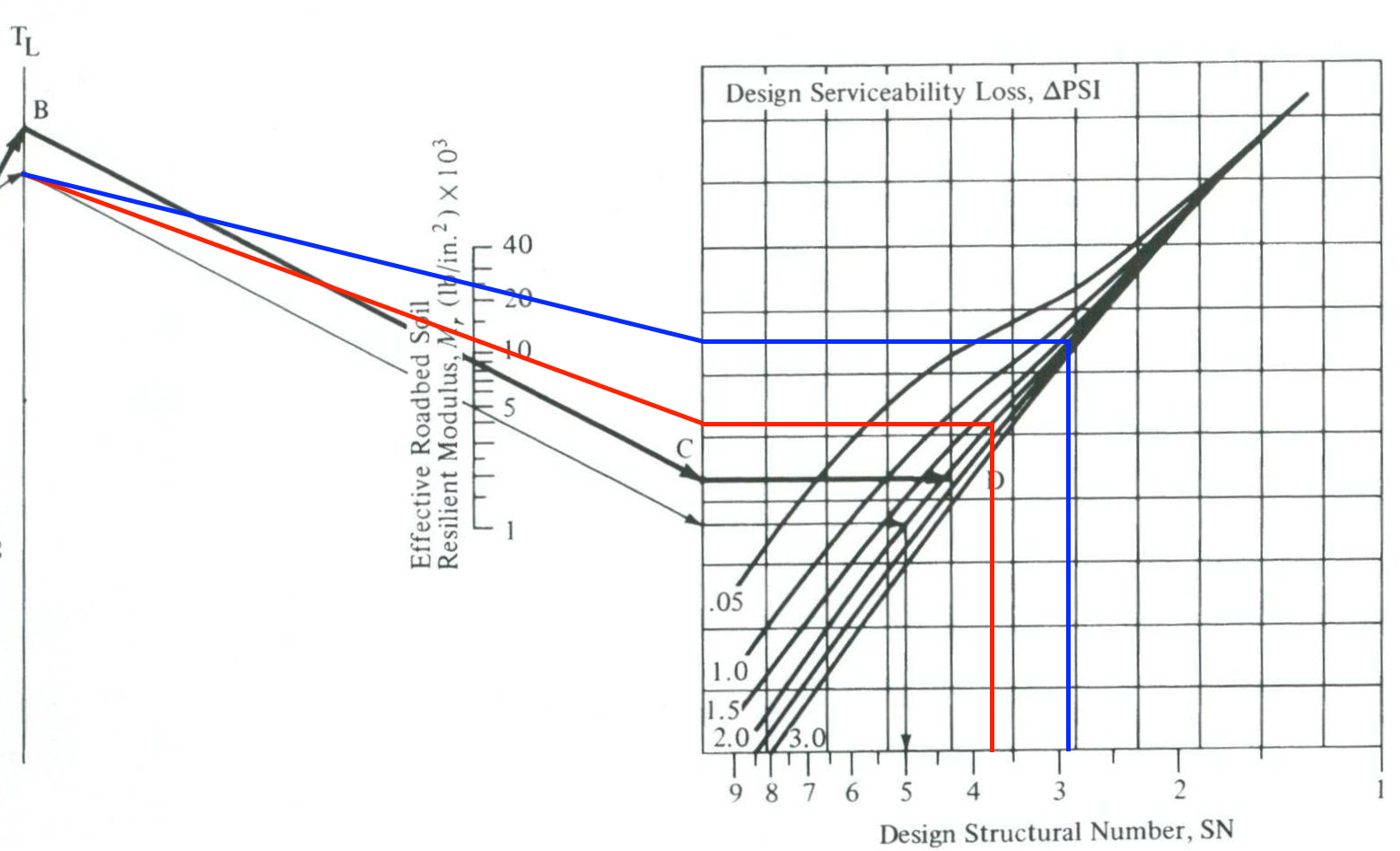
The SN for the top two layers (asphalt and base) is \(3.8\). This is the SN required to protect the subbase.
We can pick up at Step 4 again to determine the SN for the top pavement layer, which protects the base layer (shown in blue):
- Draw a line from the second \(T_L\) through the base resilient modulus value of 25 ksi to the left edge of the grid.
- Draw a horizontal line from the left edge of the grid to the curve representing the design serviceability loss of 2.0.
- Draw a vertical line dropping from the allowable PSI loss intersection down to the horizontal axis of the SN grid and read the SN.
The SN for the top layer (asphalt) is 2.8. This is the SN required to protect the base.
The SN required to protect each layer can then be used to determine the appropriate thickness for each overlying layer(s) using Equation 4.6 and solving for the depth. Start with the top layer and work down through each pavement layer.
In addition to the layer thickness calculations, there are two additional considerations when designing pavement layer thicknesses. First, AASHTO requires minimum asphalt and aggregate base thicknesses as shown in Table 4.6. Second, because the construction accuracy of contractors is limited, always round a design thickness up to the next half inch for the asphalt layer and to the next full inch for the base and subbase layers.
4.5 Pavement Management
All pavements deteriorate over time due to traffic and environmental effects (see Section 4.1.1). Pavements do not deteriorate linearly. Typically, a pavement starts out in good condition and deteriorates slowly for approximately 60-70% of its life. After that, it deteriorates more rapidly.
4.5.1 Deterioration Models
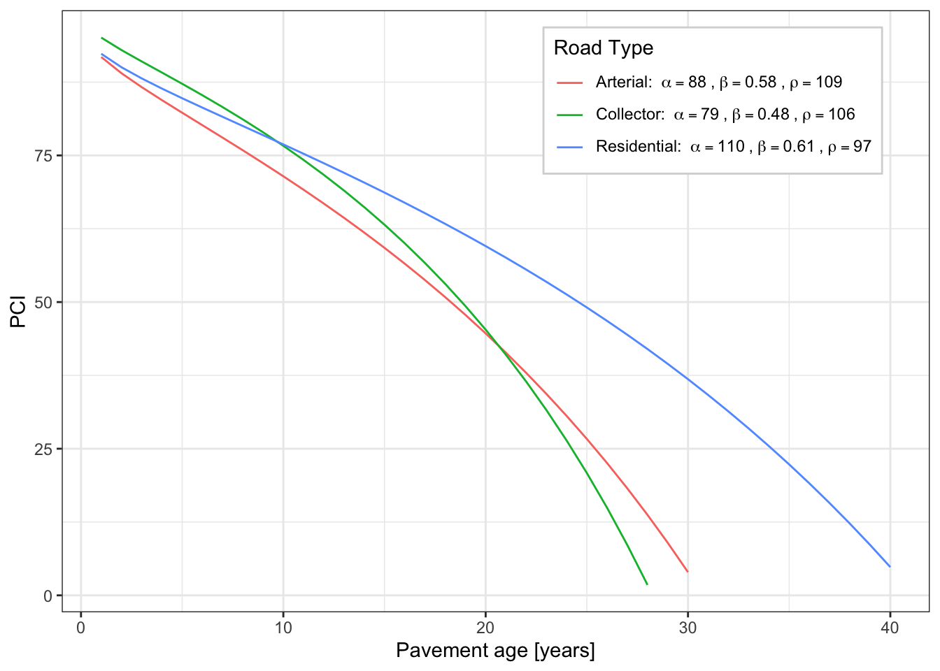
Pavement deterioration models are used to mathematically simulate how pavements will deteriorate over time. Deterioration models may vary, but those typically used in pavement management decision-support software are sigmoidal (\(S\)-shaped) of the format:
\[ PCI = 100 - \frac{\rho}{\left[\ln(\alpha/\mathrm{age})\right]^{1/\beta}} \tag{4.8}\]
where the values of the coefficients \(\alpha, \beta, \rho\) are determined empirically so the model provides a better estimate of the actual pavement deterioration. Figure 4.21 illustrates example deterioration curves estimated on arterial, collector, and residential streets in terms of the pavement condition index, or PCI.
The remaining service life (RSL) of a given pavement is the number of years for a given pavement to fall from its current condition into failed condition. Each mile of pavement loses one mile-year of service life each year.
A pavement network is a group of streets, or pavement segments, managed by an agency. Overall network health can be described in terms of an average condition index or average RSL. The average health is calculated as the average pavement condition weighted by pavement area for each street in the network. So, in terms of PCI, this is \[ PCI_{\mathrm{ave}} = \frac{\sum_i^n PCI_i \times Area_i}{\sum_i^n Area_i} \tag{4.9}\] Note that Equation 4.9 can apply to any of the condition indices in Section 4.1.2.
4.5.2 Treatments
Preventive maintenance treatments are performed on pavements in good condition. For asphalt pavements, such treatments typically include crack sealing and surface seals (slurry seal, microsurfacing, chip seal, cape seal). The primary purpose of preventive maintenance is to protect the pavement surface against moisture ingress and oxidation, which slows deterioration. Used in series, preventive treatments can significantly extend the life of a pavement and maintain it in good condition for many years.
Rehabilitation treatments are performed on pavements that are no longer in good condition. For asphalt pavements, such treatments typically include thick overlays and recycling (cold-in-place recycling, full depth reclamation). The primary purpose of rehabilitation treatments is to restore pavement to good condition.
Reconstruction is necessary when rehabilitation is not expected to be effective and involves removal of the failed pavement layers and construction of new layers.
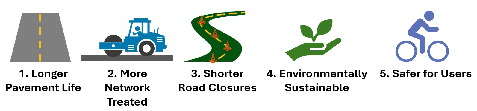
Figure 4.22 illustrates many benefits of preventive maintenance. Because preventive maintenance treatments cost less than rehabilitation treatments, a greater portion of the network can be treated annually with a fixed budget. Preventive maintenance treatments take less time to apply resulting in shorter road closures and less impact to the traveling public. Preventive maintenance is environmentally sustainable over a pavement’s life cycle because it produces less emissions and waste than rehabilitation. Improved long-term pavement condition also results in improved safety for motorists, bicyclists, and other road users.
4.5.3 Cost-effective Management Strategies
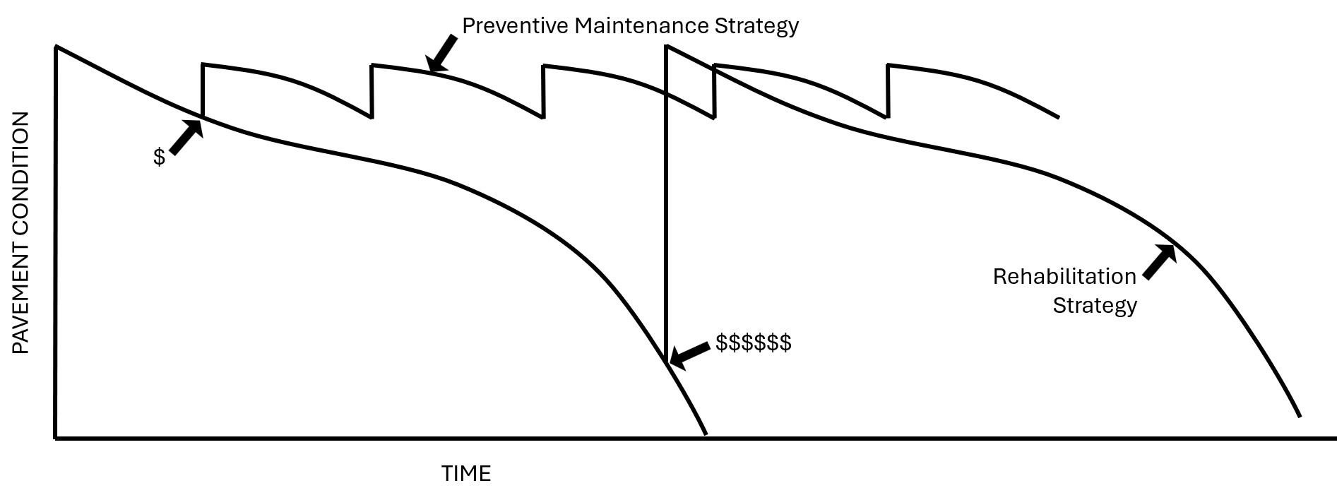
Many agencies have limited funds for pavement maintenance and rehabilitation. A common approach is to prioritize rehabilitation of the worst roads over maintenance of good roads. However, this strategy is rarely cost-effective.
The cost of performing preventive maintenance treatments while pavements are in good condition is significantly less than the cost of performing rehabilitation or reconstruction when pavements are in poor or failed condition (see Figure 4.23). Therefore, a cost-effective strategy is to find an optimal balance between preventive maintenance and rehabilitation such that the average network pavement condition is maximized, and the costs are minimized over time.
Pavement management refers to the strategic and systematic process of providing, maintaining, and improving pavement assets throughout their life cycle. It combines business and engineering principles for cost-effective resource allocation with the purpose of making defensible decisions based on quality data and analysis.
Pavement management can provide great benefits to agencies, officials, and users. Such benefits include the following:
- Improved cost-effectiveness and use of resources
- Lower long-term rehabilitation costs
- Lengthened pavement service life
- Higher levels of service and safety
- Improved performance over time
While pavement management does offer some immediate benefits, it is primarily a long-term effort and reward system.
TipMore information
Additional pavement management topics are covered in-depth in CE 566: Pavement Management
4.6 Life-Cycle Cost Analysis
All new construction, maintenance, rehabilitation, and reconstruction projects should employ an economic evaluation to identify the alternative with the best value, often defined as the least long-term cost. This practice results in defensible decisions and demonstrates wise stewardship of assets.
Life-cycle cost analysis is an economic evaluation that compares alternatives by considering all costs throughout service lives. Full service-life project costs may include design, construction, maintenance, and user costs. User costs include monetary and non-monetary elements such as delay or vehicle operating or repair costs. Salvage is the value of an asset at the end of its service life and therefore represents a monetary benefit instead of a cost. To directly compare alternatives, all project costs and values must be converted into common units.
TipReview
CCE 102 included topics on engineering economics. Those course notes can provide a review of these concepts if you need additional information.
4.6.1 Net Present Value Analysis
If the service lives of the alternatives being compared are equal, then all project costs can be converted into present worth costs. The sum of all present worth costs is the Net Present Value (NPV). Consider the cash flow diagram that transforms a future value \(F\) into its equivalent present value \(P\),
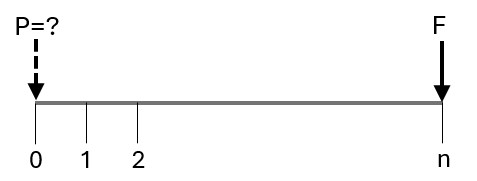
The equation that accomplishes this conversion is \[ P = \frac{F}{(1 + i)^n} \tag{4.10}\]
where \(i\) is the discount rate (usually in percent per year), and the number of compounding periods \(n\) (usually in years).
4.6.2 Annual Cost Analysis
If the service lives of the alternatives are unequal, it might be best to convert the project costs into an equivalent uniform cost. To do this, first convert all project costs into present worth costs (using Equation 4.10), and then redistributed equally to each year in the analysis period as an annuity. The cash flow diagram for this scenario is
The equation to convert a present value into an equivalent annuity is \[ A = P\frac{i (1 + i)^n}{(1 + i)^n - 1} \tag{4.11}\]
with \(A\) the reccuring annual payment and \(P, n, i\) having the same values.
Not only does concrete often have a lower life-cycle cost than asphalt, it also has a slower deterioration rate than asphalt (see Figure 4.24). Consequently, it also provides a higher level of condition throughout its service life. That said, additional factors may contribute to selecting a material type for a pavement project such as speed of construction, availability, maintenance options, etc.
4.6.3 Climate Change Adaptation
Climate affects pavements in a number of ways:
- At high temperatures, asphalt binders become softer. This leads to rutting and bleeding.
- Sunlight and UV radiation deteriorates asphalt over time.
- At low temperatures, asphalt binders become brittle, leading to cracking.
- Precipitation can introduce additional moisture to the base and sub-base layers, threatening the stability of the pavement structure.
- Freeze-thaw cycles are a major factor in cracking, buckling, and deterioration of underlying pavement layers.
- Winter road maintenance activities such as plowing and using chains or studded tires can degrade the pavement surface.
- Salting the pavement also leads to oxidation of reinforcing bars and other chemical deterioration.
As a result of these effects, pavement standards in different regions can vary substantially. Figure 4.25 shows the nine different climate zones established by CalTrans.3
Climate change therefore poses a particular challenge to pavement engineers. Hotter, drier summers may mean more rutting and bleeding, and faster pavement degradation. In many places the ground freezes solid for the entirety of winter; warming temperatures may mean that these areas will experience multiple freeze-thaw cycles in their base structure.
The impacts of climate change on transportation assets are not limited to pavements. In its Asset Management, Extreme Weather, and Proxy Indicators Pilot Project, the Arizona Department of Transportation includes a number of potential first-order and second order impacts of climate change. These effects are illustrated in Figure 4.26. Some of these effects are acute and catastrophic (such as a wildfire or a flood), while others are longer-term and more marginally damaging.
TipThink
Most pavement deterioration models in the recent literature are strictly empirical: they use past observed deterioration to forecast future deterioration. What might be the limits of this for climate change adaptation? What might pavement researchers consider?
Homework
HW 4.1: PSI Rating
Drive up and down University Ave between Cougar Blvd and University Pkwy.
- Write a description of what the drive felt and sounded like.
- If you had been on the AAHSO Road Test Committee, what would you have rated the ride quality on the PSI scale?
- Review the IRI table in the reading. What would you estimate the IRI is for this stretch of road?
HW 4.2: Distress Categorization
Group the following distresses by primary cause (environmental, traffic, material, other).
- Block cracking
- Weathering
- Pumping
- Alligator cracking
- Patching
- Corner break
- Blowups
- Spalling
- Map cracking
HW 4.3: Distress Identification
Go to the locations near campus shown on this google map and identify and photograph the primary pavement distress you see there.
HW 4.4: ESAL Comparison
se your internet browser to find the curb vehicle weight of the following four vehicles: your personal vehicle (or a friend’s if you don’t have one), a Tesla model X, a Chevrolet Tahoe, and a UTA city bus.
- Calculate the ESAL value or truck factor for each vehicle assuming the weight is carried evenly between axles.
- Compare the truck factors using a bar chart.
- How much damage does each vehicle do compared to your personal car?
CautionAssumptions
This problem requires you to make assumptions or look up values. There is not a single correct answer. Cite your sources and show your work.
HW 4.5: Annual ESALs
The one-way school bus drop-off loop at a local elementary school is used by 5 buses during the morning and afternoon routes. If the front axle carries a 9,000 lb load, and the rear axle carries 18,000 lbs, what is the annual ESAL value for the bus drop off loop? Assume 180 school days per year and that the loop is unused during the summer break.
HW 4.6: Design ESALs
The following table lists data collected from a weigh-in-motion (WIM) device in the right lane of US-6 as well as the annual growth rate expected for each axle configuration. Using a 320-day year, estimate the 25-year design ESAL value for the design lane.
| Kips | Axle Type | Count | Growth Rate |
|---|---|---|---|
| 1.5 | Single | 25000 | 0.052 |
| 1.5 | Single | 2500 | 0.022 |
| 3.5 | Single | 2500 | 0.022 |
| 3.5 | Single | 2300 | 0.022 |
| 10.0 | Single | 2600 | 0.022 |
| 12.0 | Tandem | 1300 | 0.022 |
| 20.0 | Tandem | 1500 | 0.022 |
| 34.0 | Tandem | 1500 | 0.022 |
HW 4.7: Soil Properties
You are performing a pavement design for an area with an in situ clayey material. Is this a suitable subgrade material? Why or why not?
HW 4.8: Subbase Thickness
The subgrade for a flexible pavement with a design ESAL value of 10 million has a CBR value of 5. The coefficient of relative strength for the 4-inch asphalt layer is 0.4. Below the asphalt, there are 10 inches of aggregate base, which has a coefficient of relative strength of 0.2. The coefficient of relative strength of the subbase is 0.1. Given an allowable serviceability loss of 2, what is the thickness of the subbase? Use a reliability of 95% and a standard deviation of 0.4, and assume proper drainage (\(m_2, m_3 = 1\))
TipTip
Show your answers on an included nomograph.
HW 4.9: Asphalt Thickness
You are working on a 20-year road design that has 7 million design ESALs. The state requires 90% reliability, a standard deviation of 0.4 and a change in serviceability of 1.5. The subgrade has a CBR value of 6. What is the asphalt layer thickness if the aggregate base is 12 inches thick? (Use \(a_1 = 0.4, a_2 = 0.12\).). No subbase is used, and the pavement is well-drained.
HW 4.10: Flexible Pavement Design
You are designing a pavement with a 20-year design ESAL value of 20 million and a subgrade \(M_R\) of 7.5 ksi. Local requirements include 95% reliability, a standard deviation of 0.35, and a total serviceability loss of 2 PSI. Prepare the following pavement designs:
- Design 1: Full-depth asphalt (\(M_{R1} = 380\) ksi)
- Design 2: Asphalt over aggregate base (\(M_{R1} = 380\), \(M_{R2} = 21\) ksi)
- Design 3: Asphalt over aggregate base over subbase (\(M_{R1} = 380\), \(M_{R2} = 21\), \(M_{R3} = 11\) ksi)
Given the unit weights and unit costs per ton of material, which design is the most cost-effective per lane mile? (Assume a 12-ft lane and an excavation cost of $5 per cubic yard.)
| Material | Unit weight (lb/ft$^3$) | Unit Cost ($/ton) |
|---|---|---|
| Asphalt | 140 | 100 |
| Aggregate Base | 131 | 19 |
| Subbase | 130 | 14 |
HW 4.11: A Pavement Life That Falls Short
Give three reasons why a pavement with a valid 20-year design might “fail” before 20 years.
HW 4.12: Network PCI
The tree streets in Provo were surveyed in 2022 using PCI. If the streets follow the deterioration curves described in Equation 4.8 and Figure 4.21, what is the average network PCI in 2025? All roads are 32 ft wide.
| ID | Street | Begin | End | Functional Class | Length (ft) | 2022 PCI |
|---|---|---|---|---|---|---|
| 1 | Aspen Ave | Birch | Cul de sac | Residential | 924 | 90 |
| 2 | Ash Ave | Birch | Locust | Residential | 1254 | 92 |
| 3 | Briar Ave | Birch | Locust | Residential | 1601 | 86 |
| 4 | Birch Ln | Briar | Aspen | Residential | 925 | 65 |
| 5 | Cherry Ln | Cedar | Briar | Residential | 354 | 56 |
| 6 | Cherry Ln | Briar | Aspen | Residential | 777 | 89 |
HW 4.13: Treatment Selection
Use the Pavement Treatment Toolbox at https://roadresource.org/ to answer the following questions.
- An urban arterial street with a PCI of 45 has moderate to severe alligator cracking and moderate rutting. The road has a history of drainage issues and is subject to freeze-thaw cycles. Recommend a cost-effective treatment that would effectively address these issues, describe the treatment in your own words, and justify your recommendation.
- A rural residential road with a PCI of 78 has a longitudinal crack along the construction joint and weathering (called oxidation on roadresource.org). Recommend a cost-effective treatment that would maintain the pavement condition for 8-10 years, describe the treatment in your own words, and justify your recommendation.
HW 4.14: Remaining Service Life
Each mile of pavement loses one year of service life each year. This means that for a 650-lane mile network (such as the City of Provo’s), 650 lane-mile-years of service life are used up each year. To maintain the average RSL, the city must add at least 650 lane-mile-years of service life through maintenance each year. Use roadresource.org’s RSL calculator to answer the following questions for a network size of 650 lane-miles and a $1M budget.
- If the entire budget was spent on crack sealing, how many lane miles can be treated? How many lane-mile-years of service life does this add to the network?
- If the entire budget was spent on slurry seals, how many lane miles can be treated? How many lane-mile-years of service life does this add to the network?
- If the entire budget was spent on major mill and fill, how many lane miles can be treated? How many lane-mile-years of service life does this add to the network?
- Optimize the combination of crack, slurry, and mill and fill treatments such that the RSL is maintained (approx. 650-lane-mile-years added to the network). This should balance preventive maintenance (crack and slurry) and rehabilitation (mill and fill) efforts, such that the budget is not exceeded.
HW 4.15: Maintenance LCCA
You have just constructed a new asphalt pavement and are considering maintenance options over the next several decades.
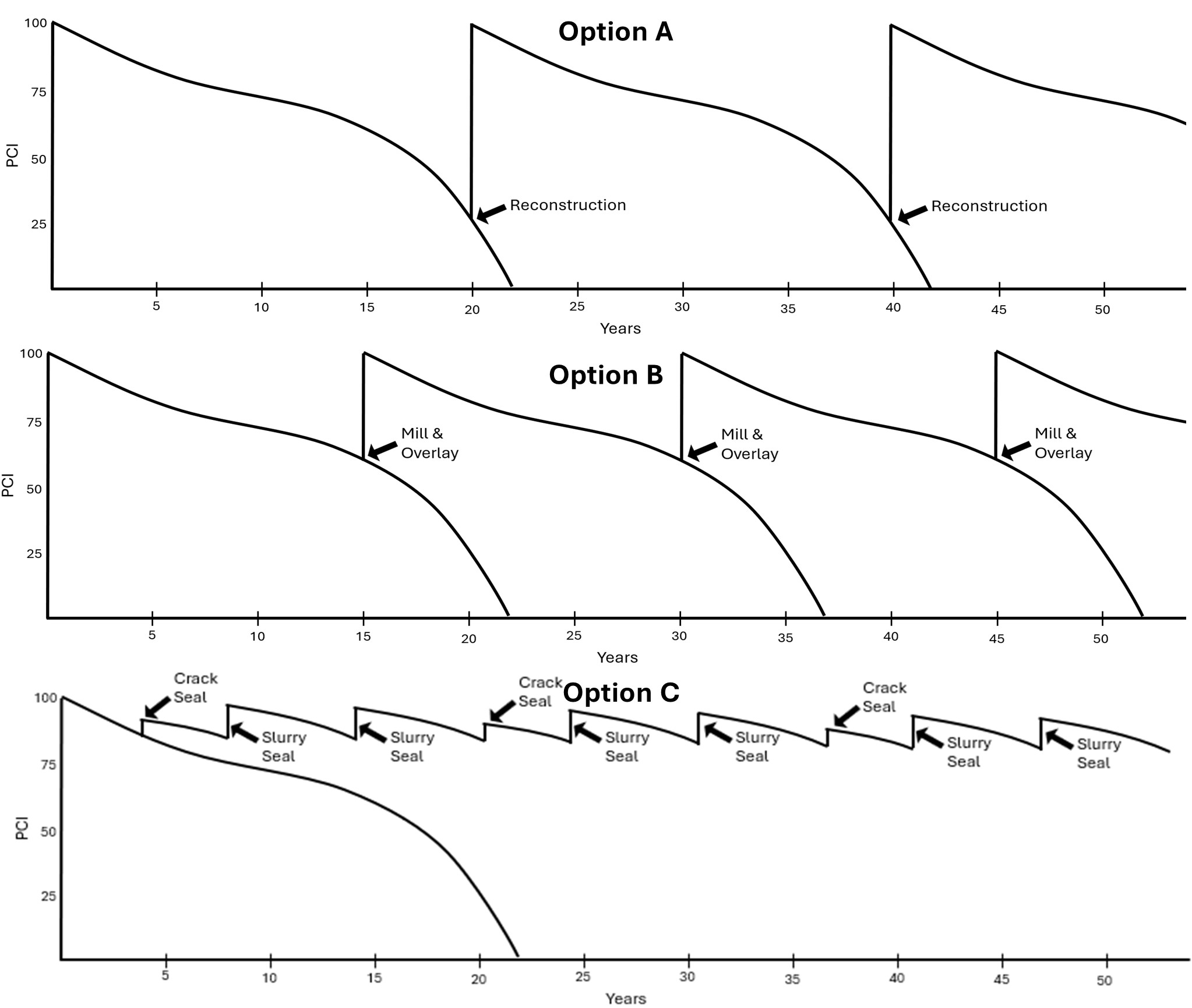
- Option A is to perform a reconstruction of the section every 20 years when the pavement falls into failed condition.
- Option B is to perform a thin mill and overlay every 15 years while the pavement is in fair condition.
- Option C is to perform a crack seal after 4 years followed by a series of slurry seals and crack seals as shown in the figure.
Crack seals extend the pavement life by 4 years while slurry seals extend the pavement life by 6 years. The treatment costs in each year for all three options are provided in the table below, followed by a figure of the expected PCI under each treatment plan.
| Option | Year | Treatment | Cost |
|---|---|---|---|
| A | 20 | Reconstruction | $1,050,609 |
| 40 | Reconstruction | $2,090,489 | |
| 60 | $ - | ||
| B | 15 | Thin Mill & Overlay | $353,834 |
| 30 | Thin Mill & Overlay | $592,795 | |
| 45 | Thin Mill & Overlay | $993,138 | |
| 60 | $ - | ||
| C | 4 | Crack seal | $8,079 |
| 8 | Slurry seal | $27,811 | |
| 14 | Slurry seal | $34,187 | |
| 20 | Crack seal | $14,008 | |
| 24 | Slurry seal | $48,224 | |
| 30 | Slurry seal | $59,279 | |
| 36 | Crack seal | $24,290 | |
| 40 | Slurry seal | $83,620 | |
| 46 | Slurry seal | $102,790 | |
| 52 | $ - |
Complete the following:
- Perform an LCCA for the three maintenance options using an interest rate of 3.5%. Run Option A through 60 years, Option B through 60 years, and Option C through 52 years. Do not include a treatment in the final analysis year for any option.
- Which maintenance option is the most cost-effective?
- Which maintenance option provides the highest pavement condition throughout the life cycle? (No calculations required; a simple visual interpretation of the figure is sufficient.)
HW 4.16: Rehabilitation LCCA
One benefit of full-depth reclamation is that the occurrence and severity of potholes is significantly reduced throughout the pavement’s service life. A local City is considering the following options for rehabilitating a residential neighborhood with 5.2 centerline miles of streets (one 12-ft lane in each direction).
Option A is to perform a 3-inch asphalt mill and overlay throughout the neighborhood at a cost of $48 per square yard (yd\(^2\)). This initial construction will result in a user cost (inconvenience due to detours, and delays) of $0.20/yd\(^2\). Eight years after construction, a microsurfacing seal treatment will be performed at cost of $9/yd\(^2\). Starting in year 12, the City will need to spend $0.16/yd\(^2\)per year to repair potholes. Those same potholes will cost users $0.04/yd\(^2\)per year in vehicle damage. At the end of a 20-year period, the pavement will have a salvage value of $5/yd\(^2\).
Option B is to perform FDR with a 3-inch asphalt concrete surface throughout the neighborhood at a cost of $57/yd\(^2\). This initial construction will take longer than a traditional mill and overlay and will therefore result in a user cost of $0.25/yd\(^2\). Eight years after construction, a slurry seal will be performed at a cost of $3/yd\(^2\). The FDR stabilization postpones pothole occurrence and reduces the severity such that the City only spends $0.08/yd\(^2\)on pothole repairs in year 15 and 18. The corresponding user cost for pothole damage in those same years is $0.02/yd\(^2\). At the end of the 20-year period, the pavement will have a salvage value of $20/yd\(^2\).
- Draw the cash flow diagrams for the two options.
- Perform a life cycle cost analysis for the two options using an interest rate of 3.5%
- Which rehabilitation option is the most cost-effective?
HW 4.17: Life Cycle Cost Analysis
You are conducting a LCCA analysis for a new rural highway. Using observations from other similar roads in the same climate region, you have estimated the following pavement deterioration function: \[PCI_n = PCI_0 - 90\exp(-8/n)\] where \(n\) is the number of years since the last treatment and \(PCI_0\) is the initial pavement condition index after the last treatment. You have the following treatment options:
- A full-depth reconstruction of the road returns the PCI to 100, and costs $400M
- An in-place surface recycling adds 15 PCI to the previous year’s PCI and costs $100M
- A HMA overlay adds 7 PCI to the previous year and costs $30M
- A seal coat adds 2 PCI and costs $5M.
In year 20, any PCI over 70 is considered recovered cost. That is, if \(PCI_{20} > 73.5\), add a positive cash flow of $3.5 M in year 20. But for any year where the PCI is below 70, the difference is considered an expenditure (if the PCI is 68 in a year, add a 2 M deficit). For each plan, plot the expected PCI in each year and calculate the NPV. Use a discount rate of 4%. Consider the following treatment plans:
- Full-depth reconstruction in year 0. No additional treatments. Hint: your NPV should be $520-540 M.
- Full-depth reconstruction in year 0, HMA overlay in year 6, in-place recycling in year 11, and a seal coat in year 16.
- Design your own pavement treatment plan, trying to minimize the Net Present Value (NPV).
HW 4.18: Climate Change Adaptation
Re-calculate the \(NPV\) and \(PCI\) values from your plans above, assuming that the value of the \(e\) coefficient changes from 8 to 6.5 as a result of warmer temperatures in your region. What impact would this have on the sustainability of your pavement plans? Do your plans still have the same ordering of NPV?